Themes and Arranging Plots
Data Visualization and Exploration
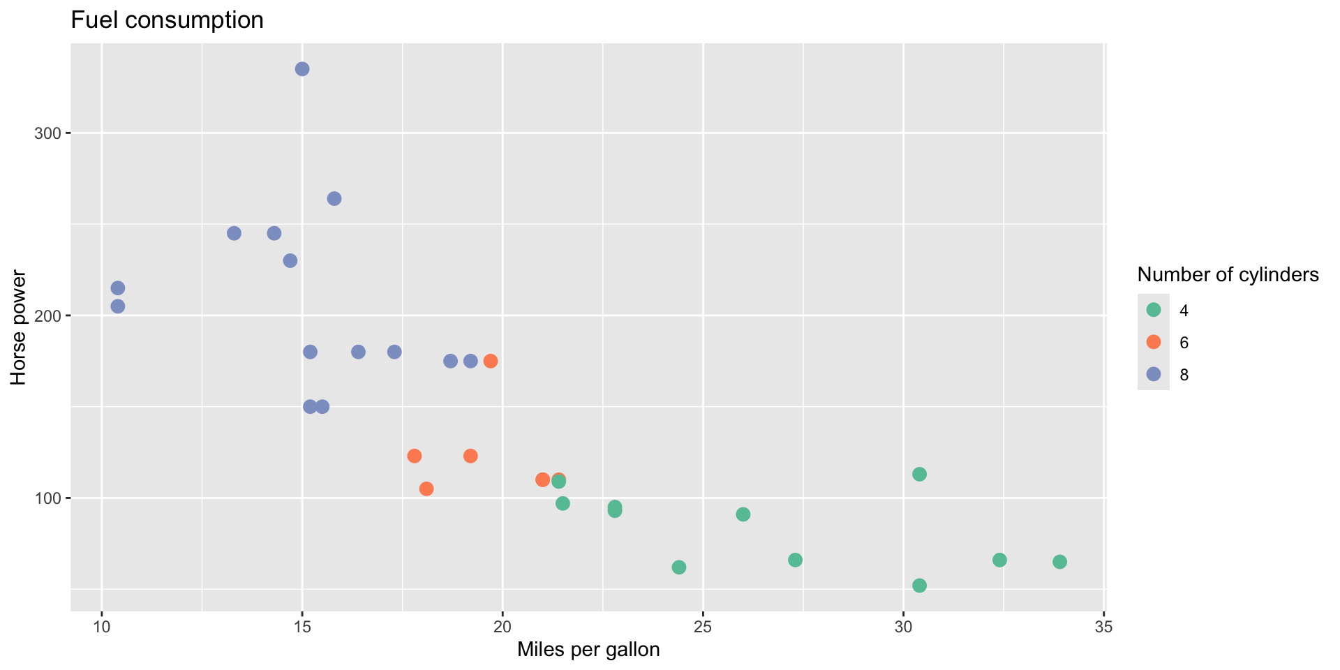
A tour of built-in themes
A tour of built-in themes
A tour of built-in themes

A tour of built-in themes
A tour of built-in themes
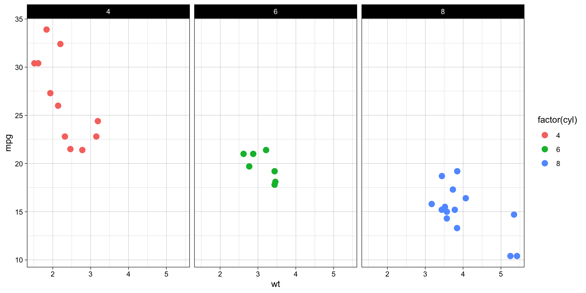
A tour of built-in themes
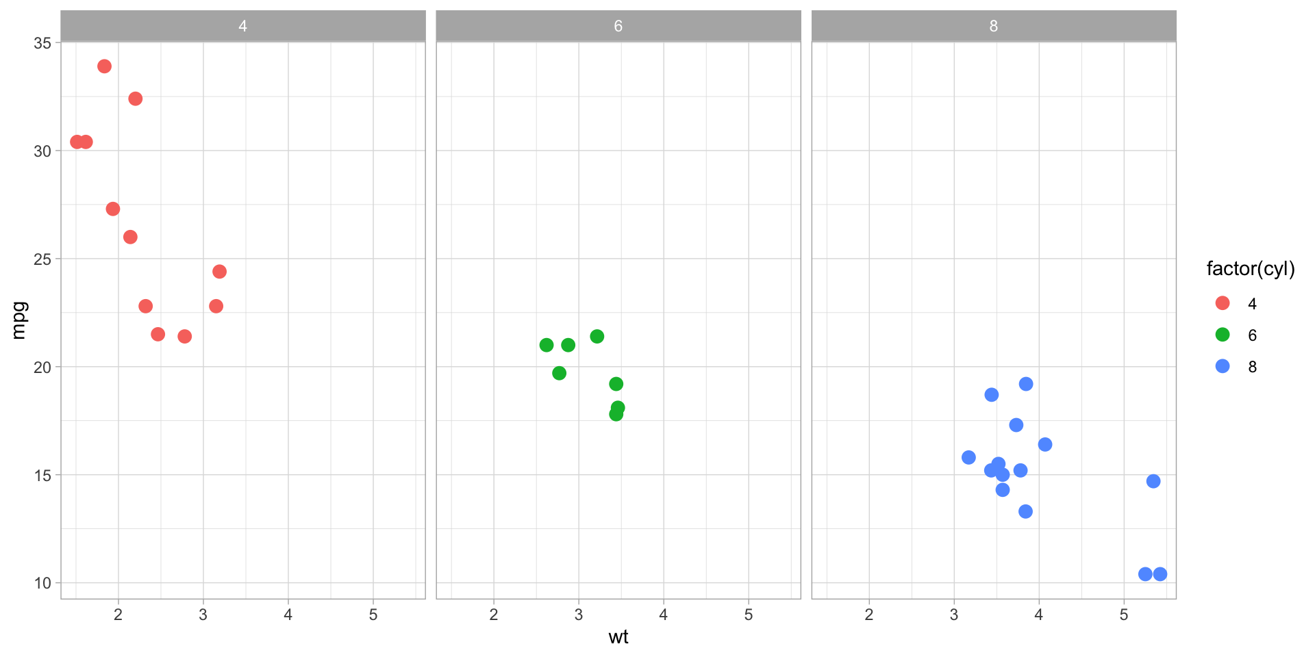
A tour of built-in themes
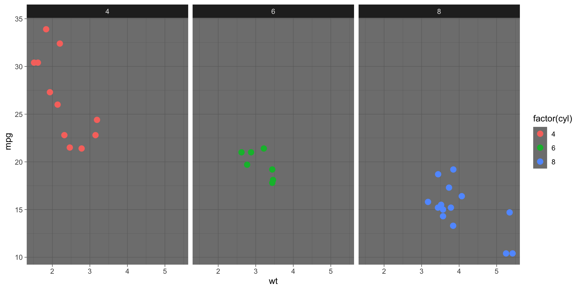
A tour of built-in themes
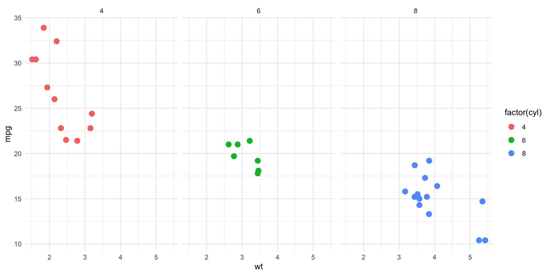
A tour of built-in themes
A tour of built-in themes
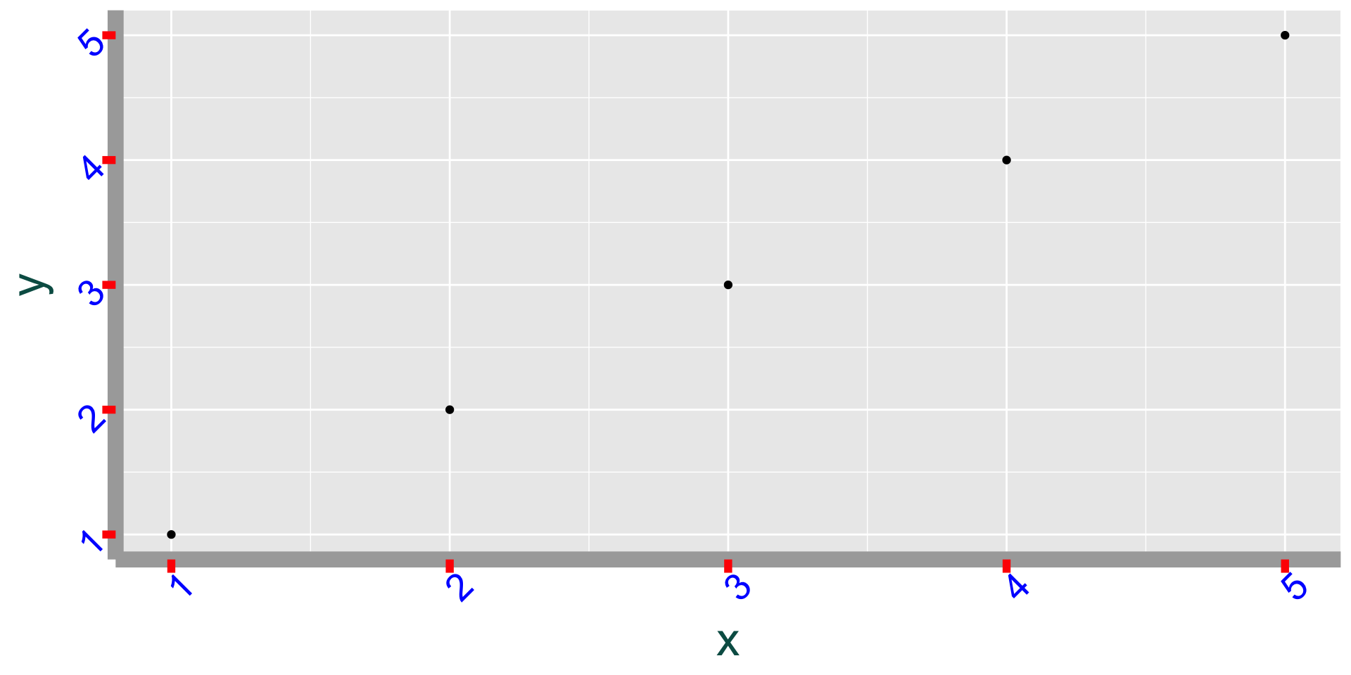
Element functions:
element_text()

Element functions:
element_text()
Element functions:
element_text()
Element functions:
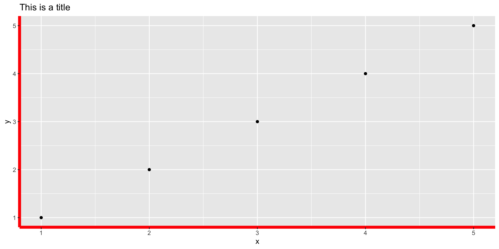
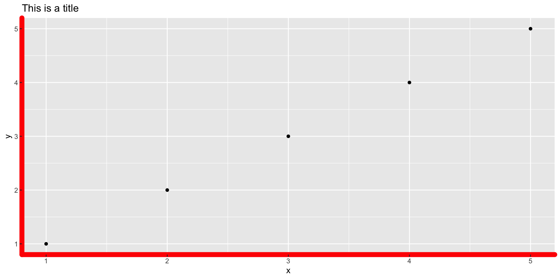
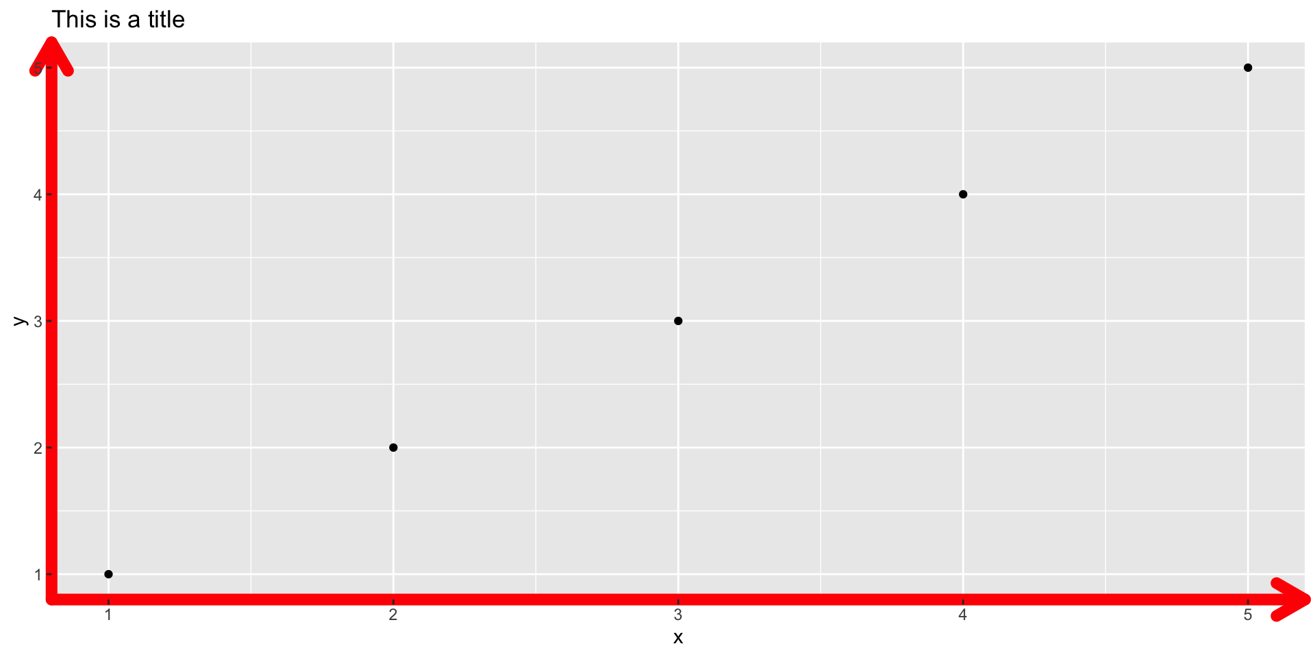
element_line()

Element functions:
element_line()
Element functions:
element_line()
Element functions:
element_line()
Element functions:
element_rect()
Element functions:
element_rect()
Element functions:
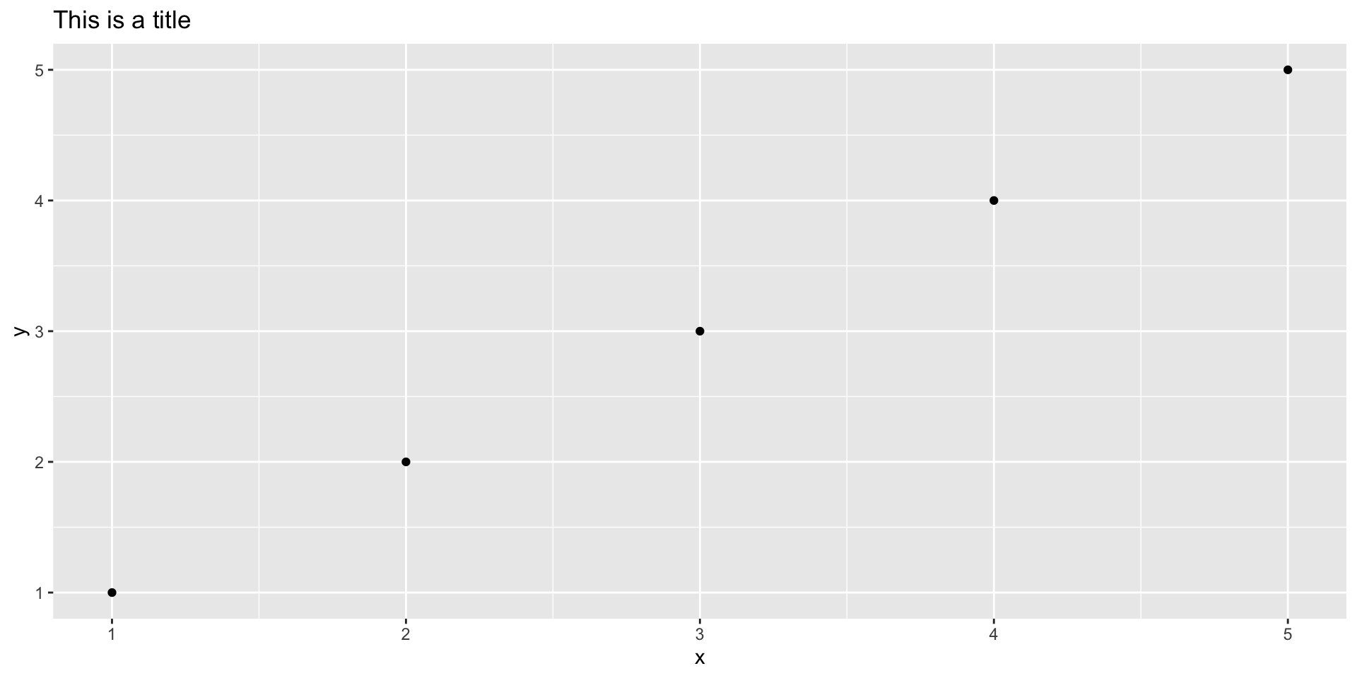
element_blank()

Element functions:
element_blank()
Element functions:
element_blank()
Element functions:
element_blank()

Theme elements
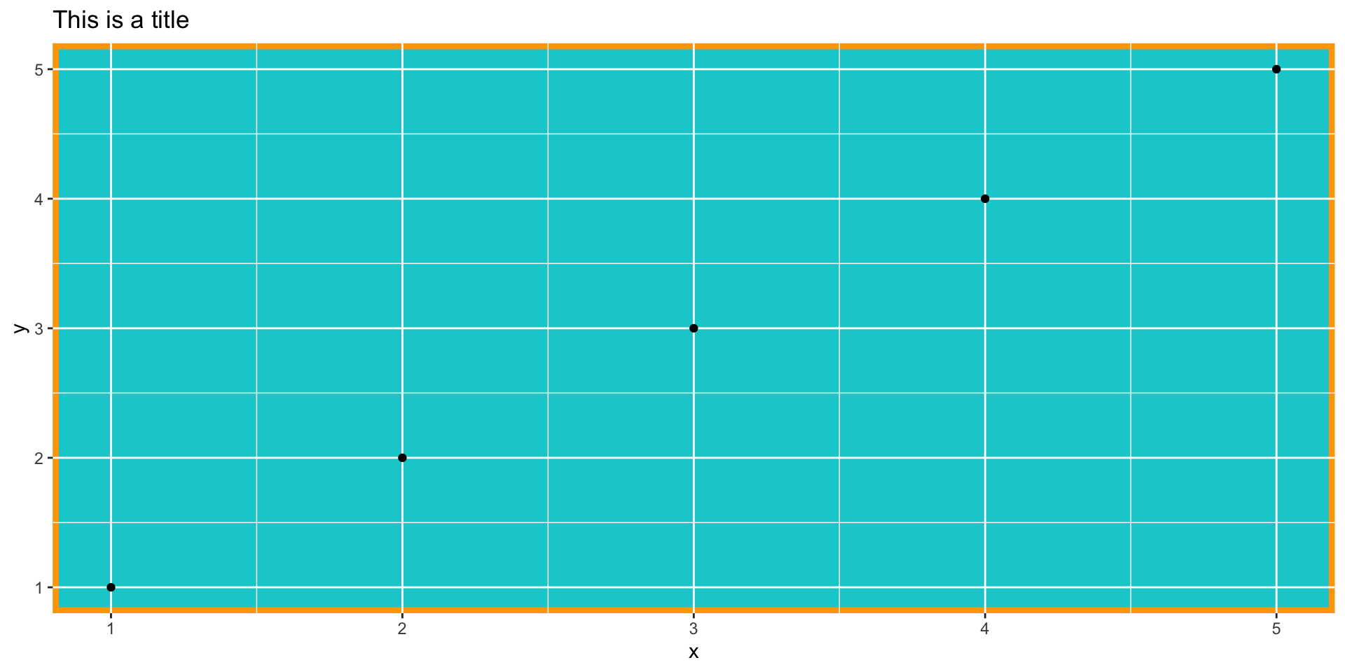
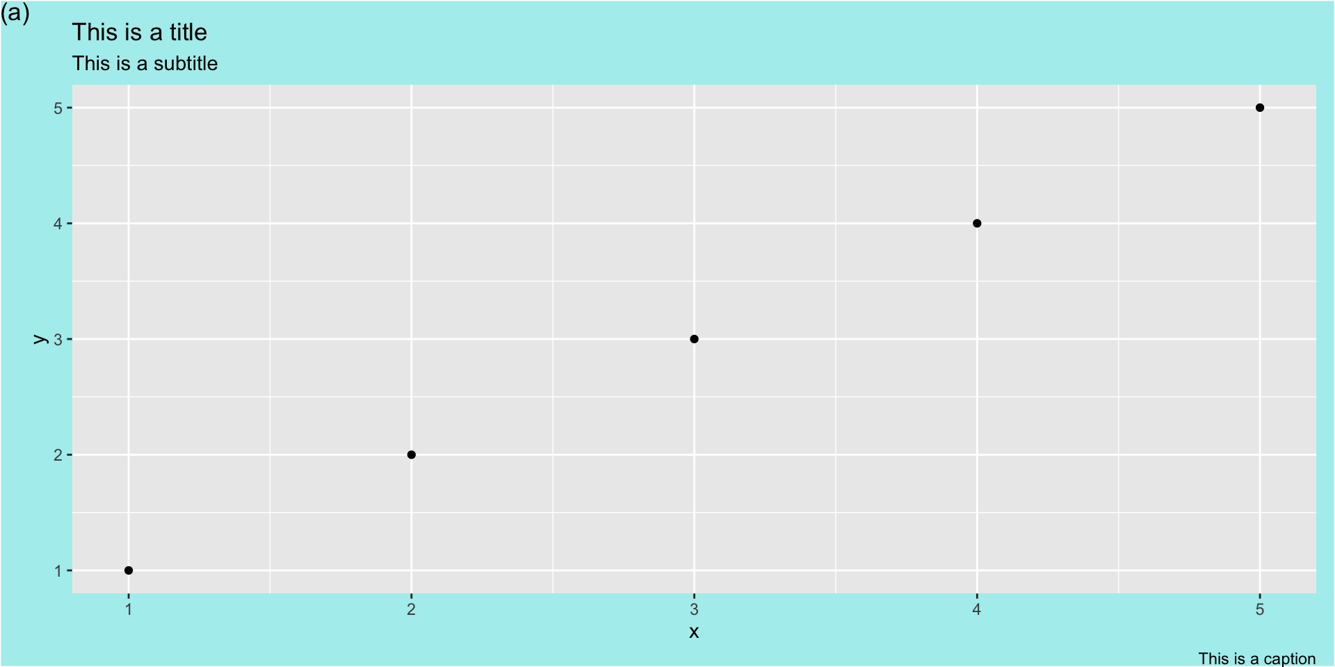
Plot elements
plot.backgroundplot.titleplot.title.positionplot.captionplot.caption.positionplot.tagplot.tag.positionplot.margin
Theme elements
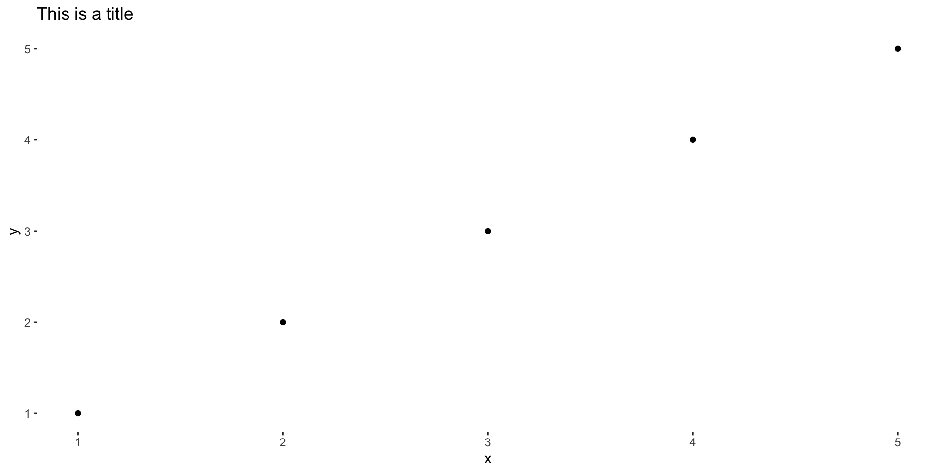
Axis elements
Theme elements
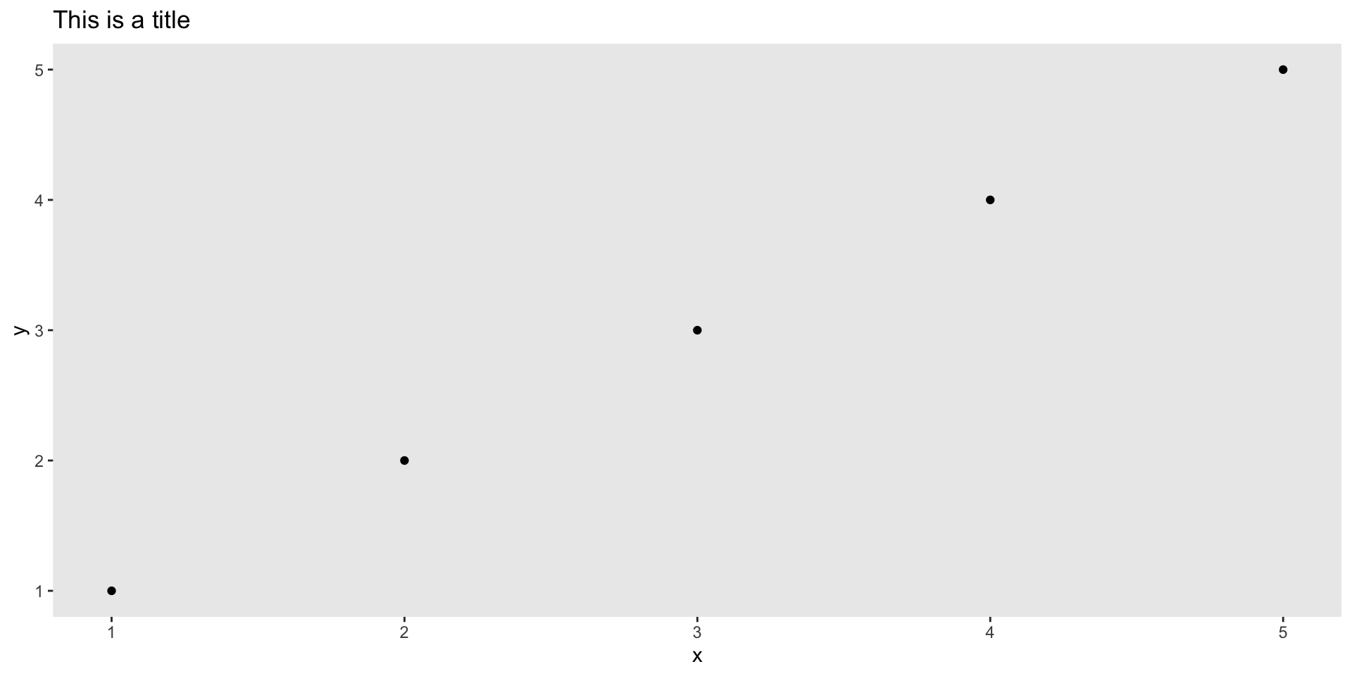
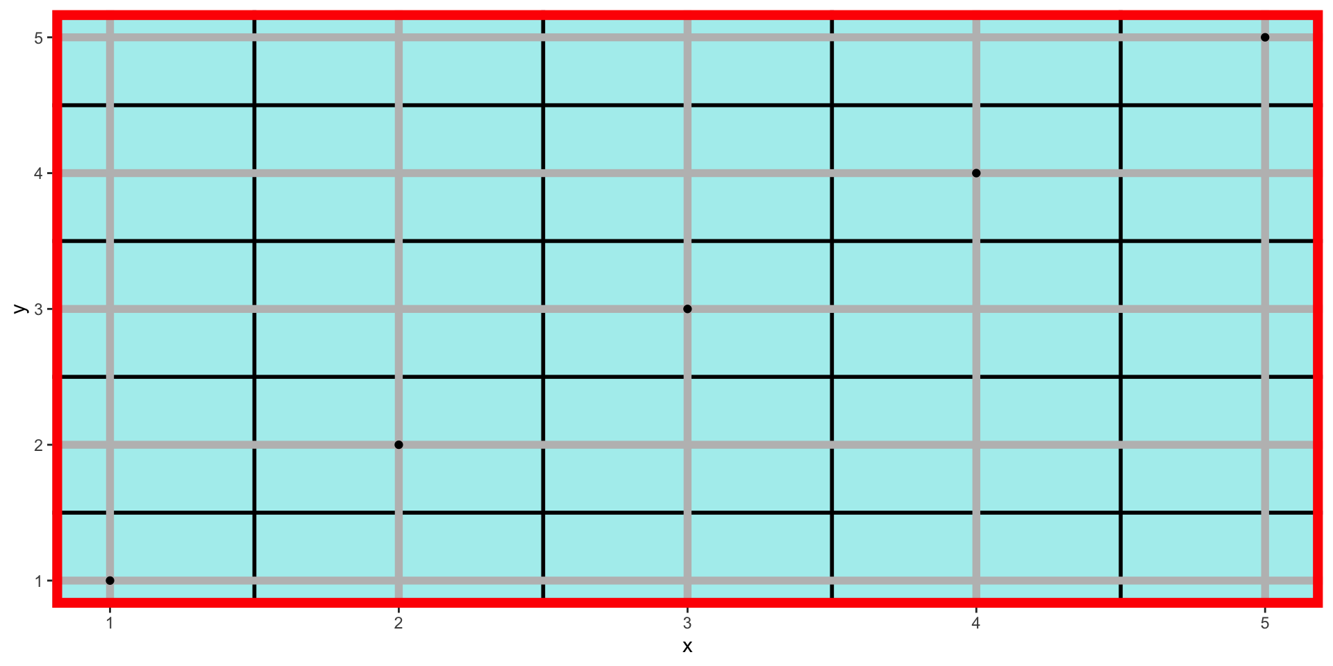
Panel elements
panel.backgroundpanel.borderpanel.gridpanel.grid.majorpanel.grid.minorpanel.grid.major.xpanel.grid.major.ypanel.grid.minor.xpanel.grid.minor.y
Theme elements
Legend elements
legend.background
legend.margin
legend.spacing
legend.spacing.x
legend.spacing.y
legend.key
legend.key.size
legend.key.height
legend.key.width
legend.text
legend.text.align
legend.title
legend.position
legend.direction
legend.justification
legend.box
legend.box.just
legend.box.margin
legend.box.background
legend.spacing
ggplot(df,aes(x,y,color=factor(x))) +
  geom_point(size=10) +
  theme(legend.key=element_rect(colour = "red",fill="blue"),
        legend.background = element_rect(fill="darkolivegreen4"),
        legend.margin = margin(5,5,5,40),
        legend.text=element_text(size=20),
        legend.title = element_text(family="Times",hjust = 1),
        legend.position = "top")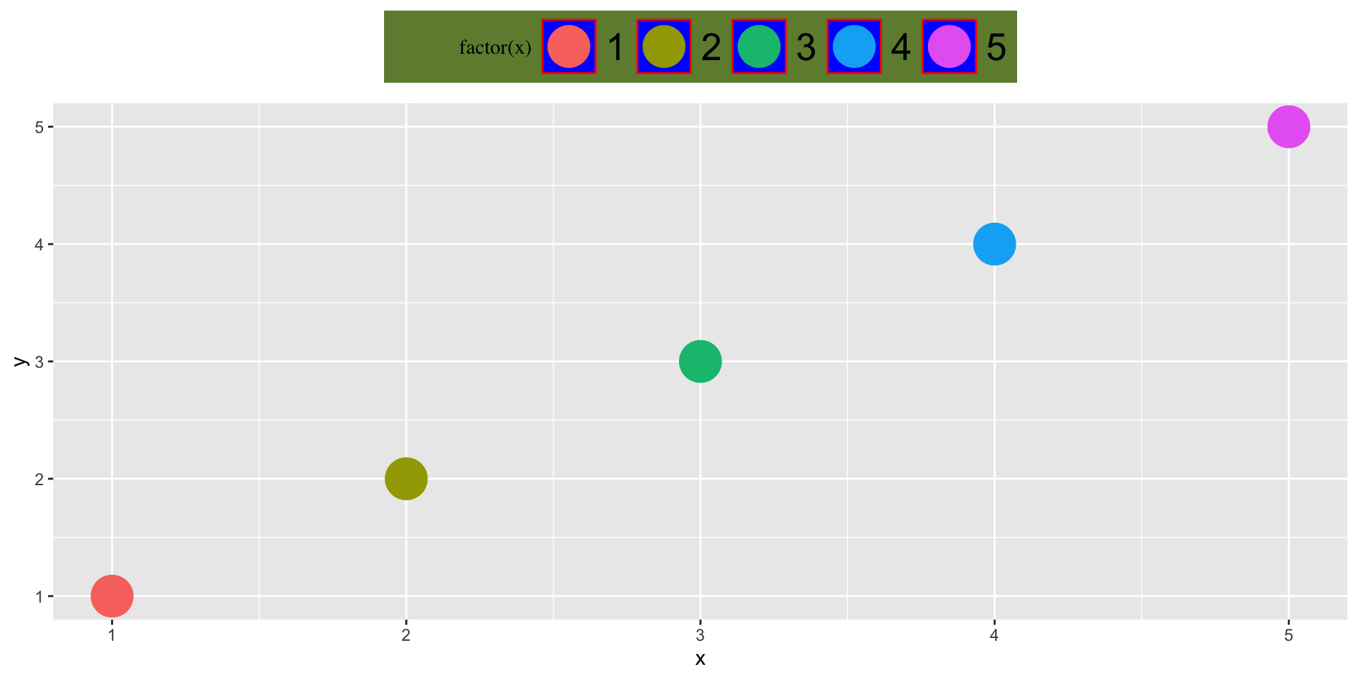
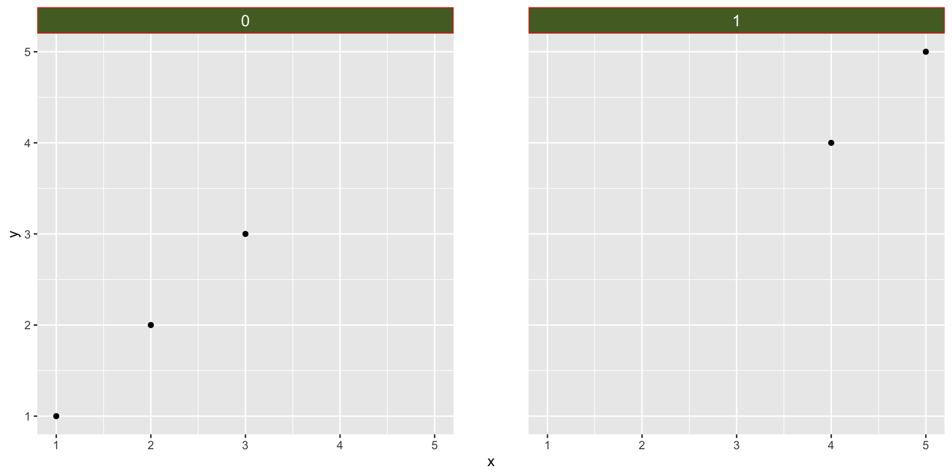
Facet elements
Panel elements
panel.backgroundpanel.background.xpanel.background.ypanel.placementstrip.textstrip.text.xstrip.text.ystrip.switch.pad.gridstrip.switch.pad.wrappanel.spacingpanel.spacing.xpanel.spacing.y
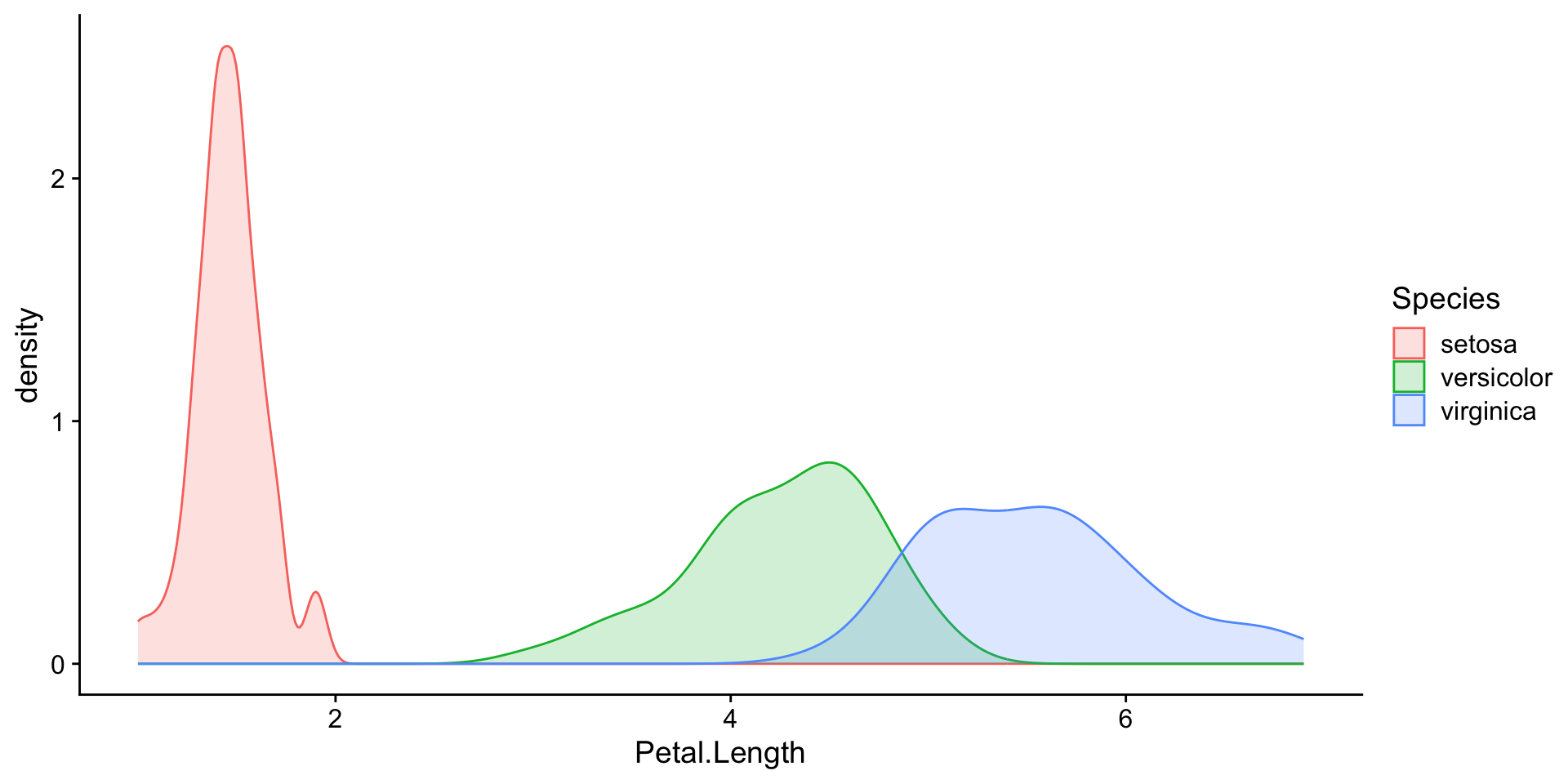
Creating your own custom theme
Creating your own custom theme
p + theme_light(base_size=10, base_family = "Courier") +
  theme(panel.border = element_blank(),
        panel.grid.minor.x = element_blank(),
        axis.ticks = element_blank(),
        legend.position = "top",
        axis.title.x = element_text(margin=margin(t=10)),
        axis.title.y = element_text(margin=margin(r=10)),
        legend.text=element_text(margin=margin(0,10,0,0)),
plot.title = element_text(face="bold")) 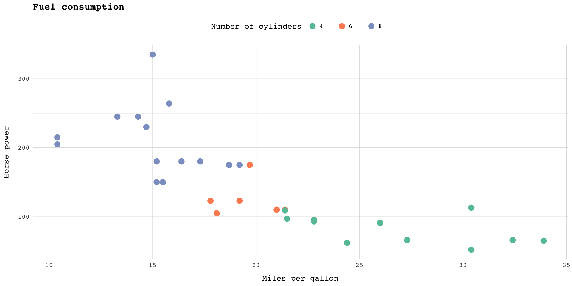
Creating your own custom theme

Arranging plots in a grid
Arranging plots in a grid
Arranging plots in a grid
Arranging plots in a grid
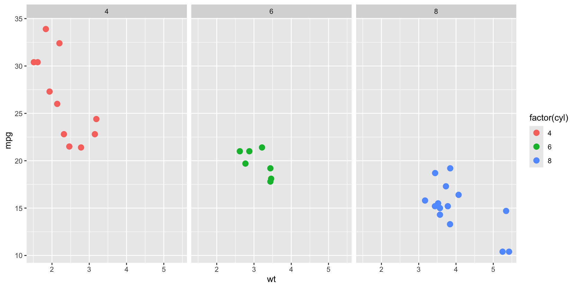
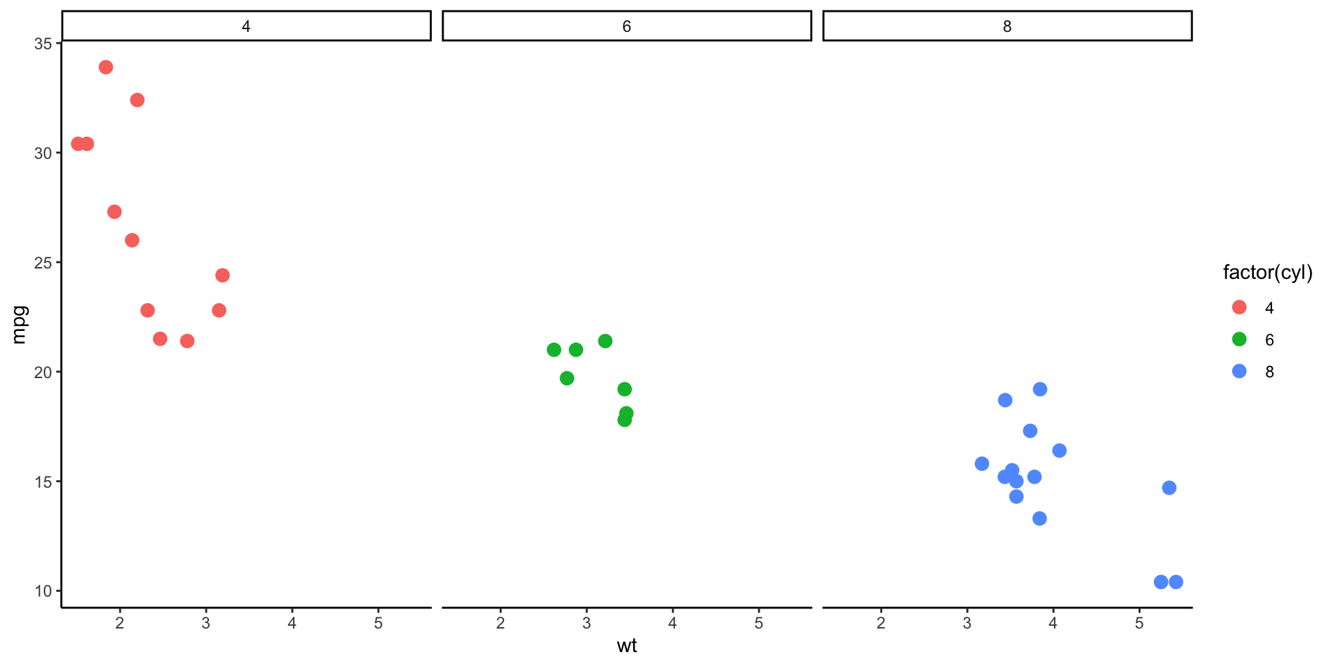
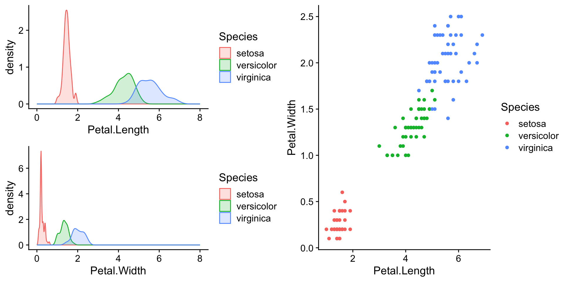
We can put the plots in a grid, aligning them on the x axis, appropriately changing the scales.
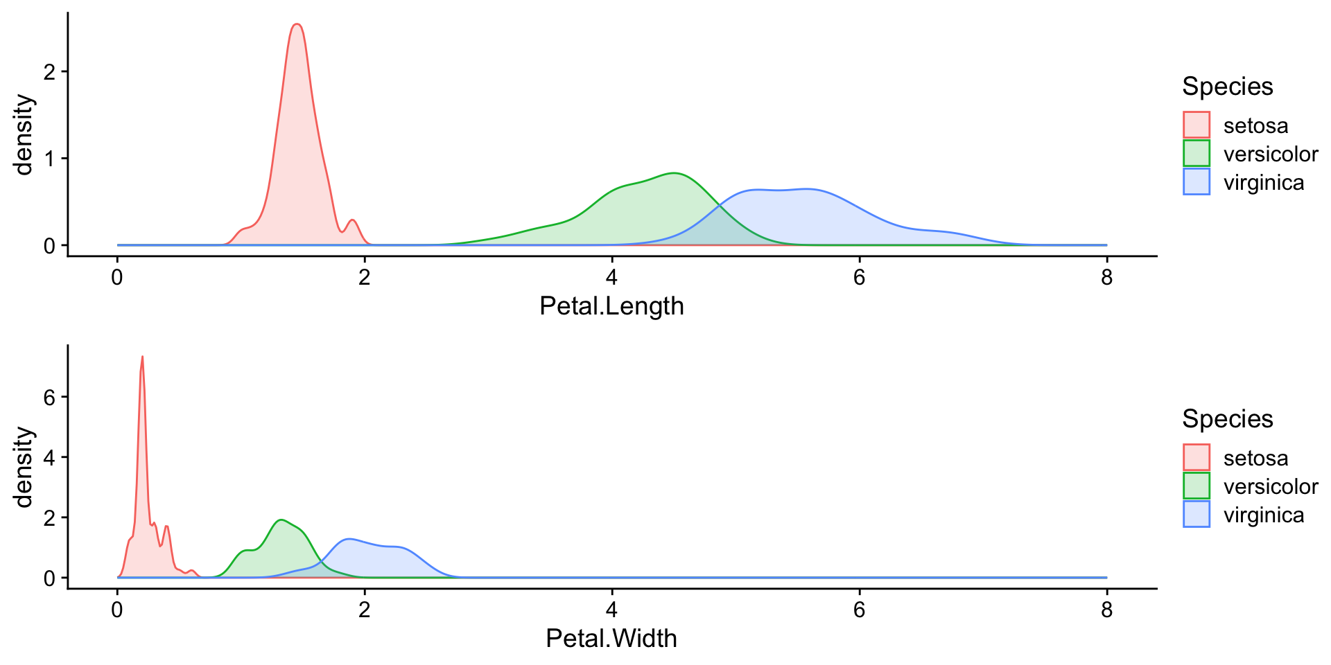
Arranging plots in a grid
We can put the plots in a grid, aligning them on the x axis, appropriately changing the scales.

Arranging plots in a grid
We can put the plots in a grid, aligning them on the x axis, appropriately changing the scales.
Arranging plots in a grid
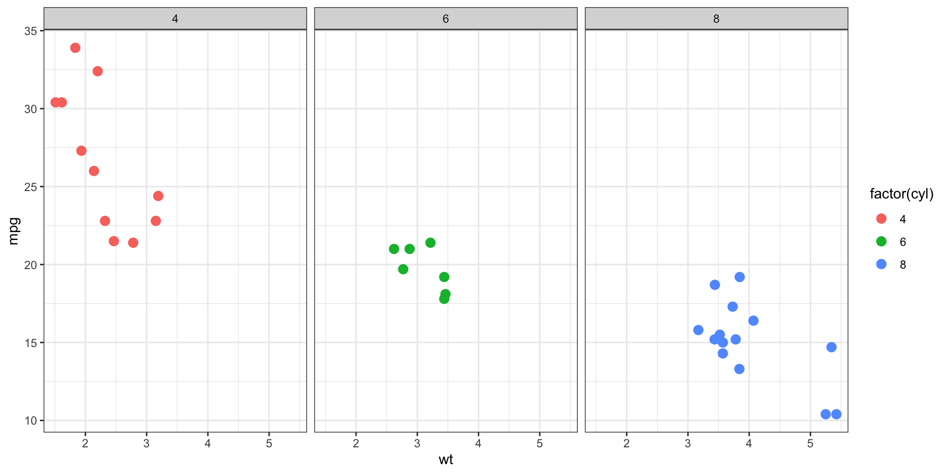
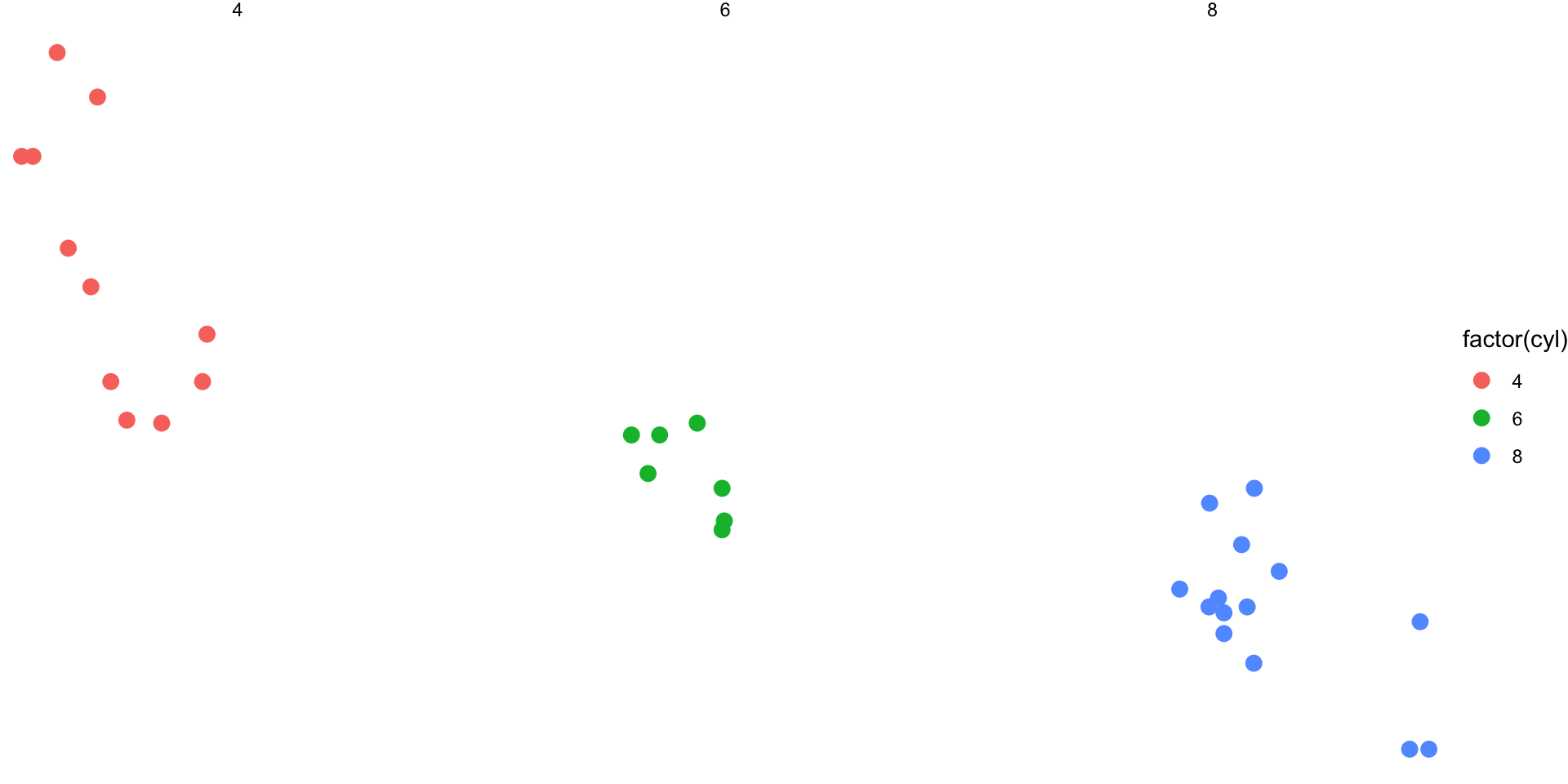
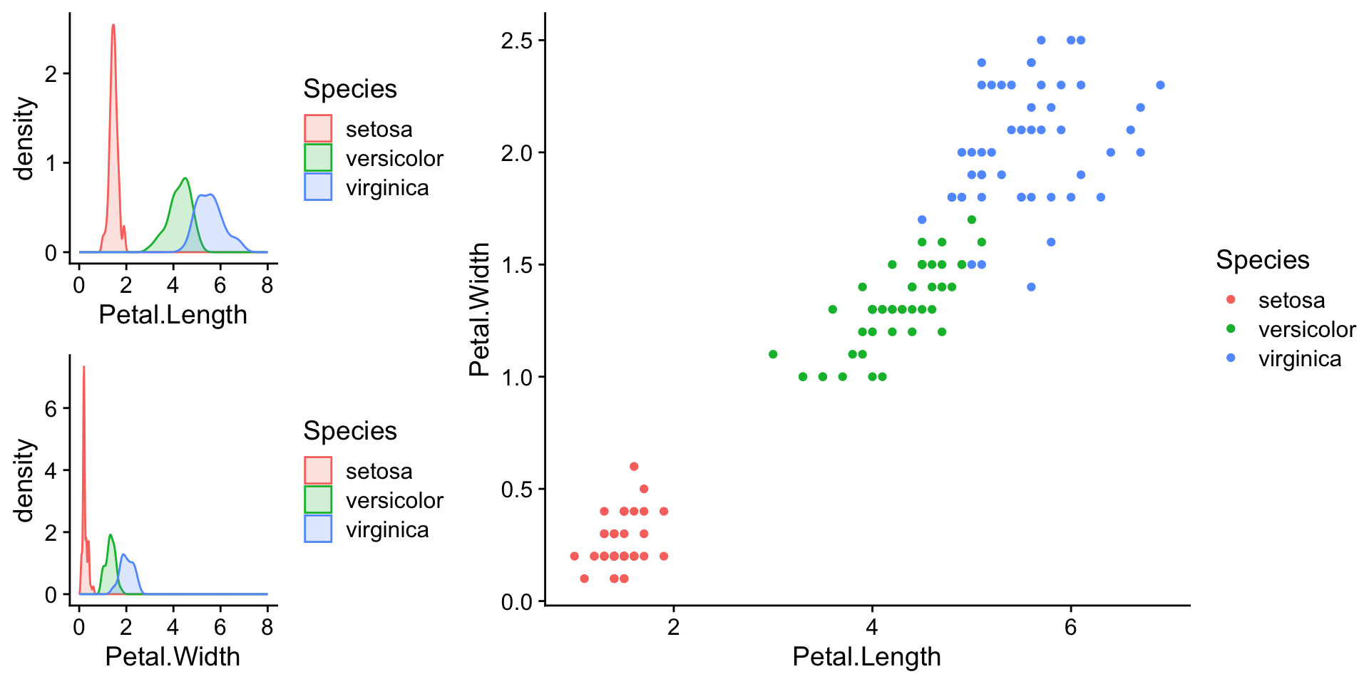
We can use NULL to leave “holes” in the tables.
Arranging plots in a grid
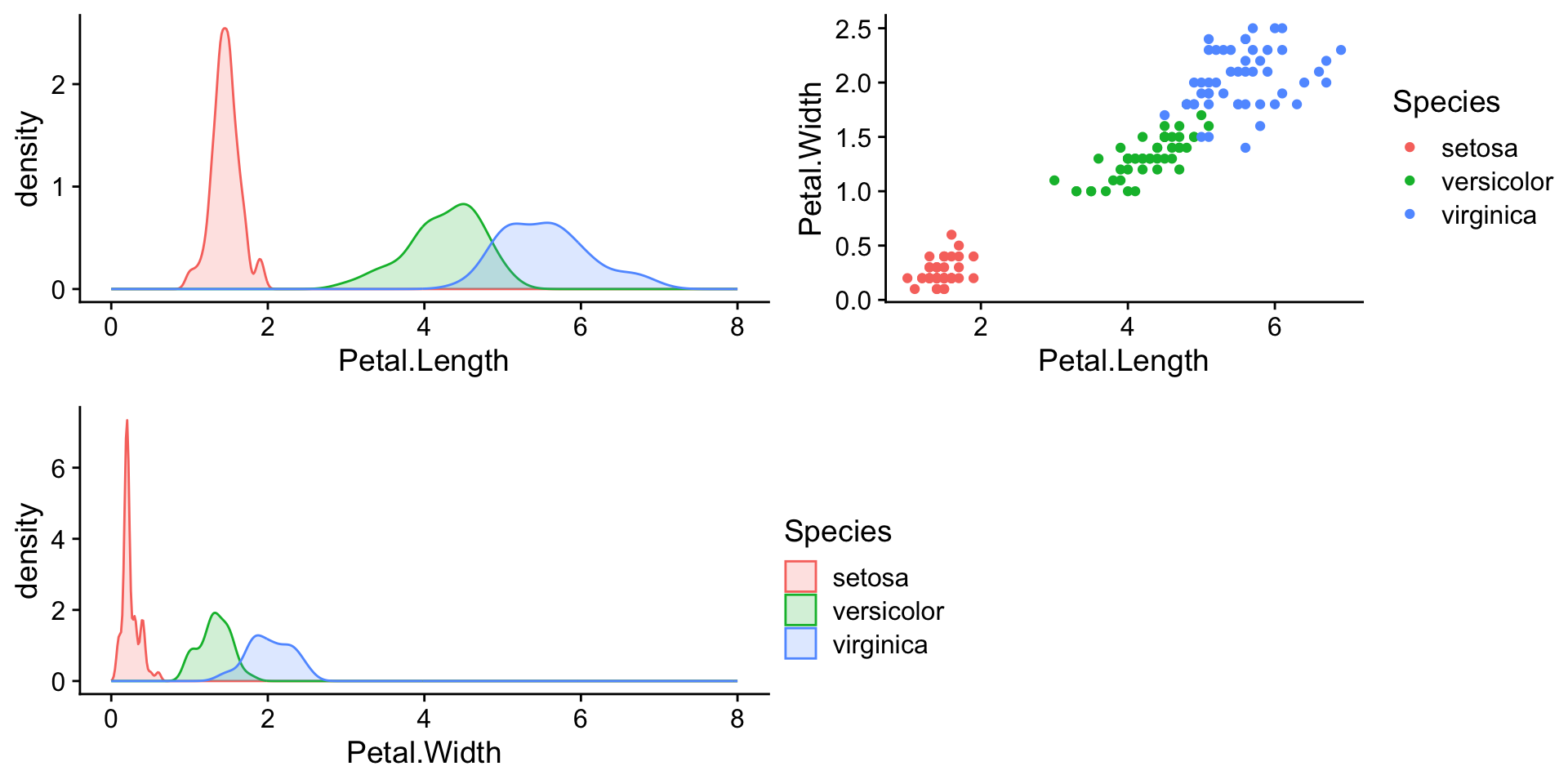
We can also nest grids into one another, to create more complex arrangements.
Arranging plots in a grid
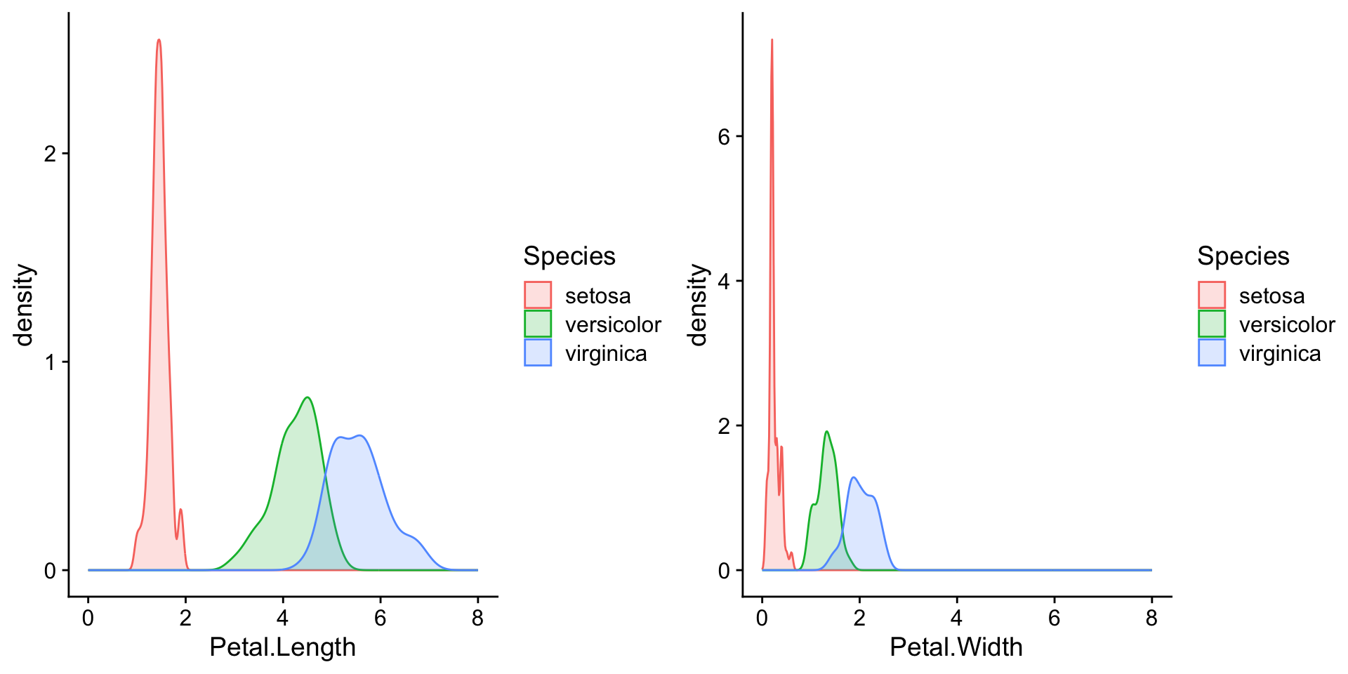
And adjust the widths
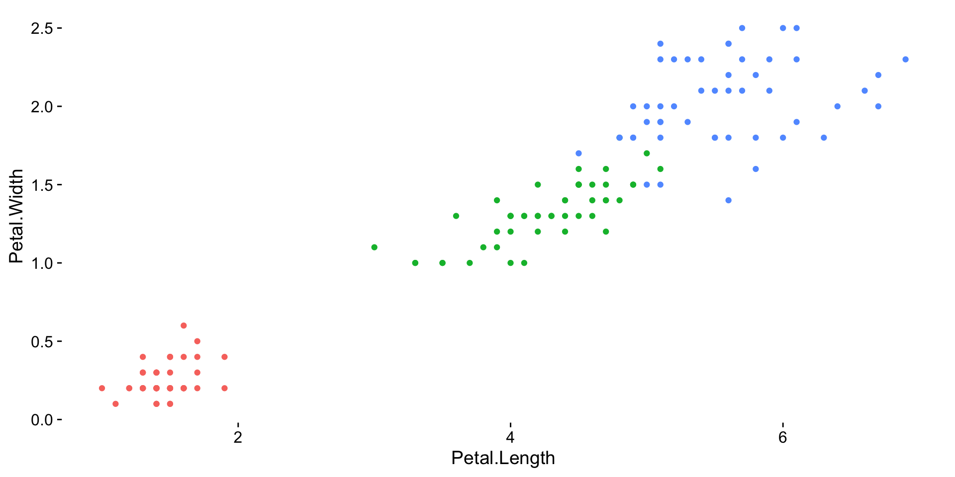
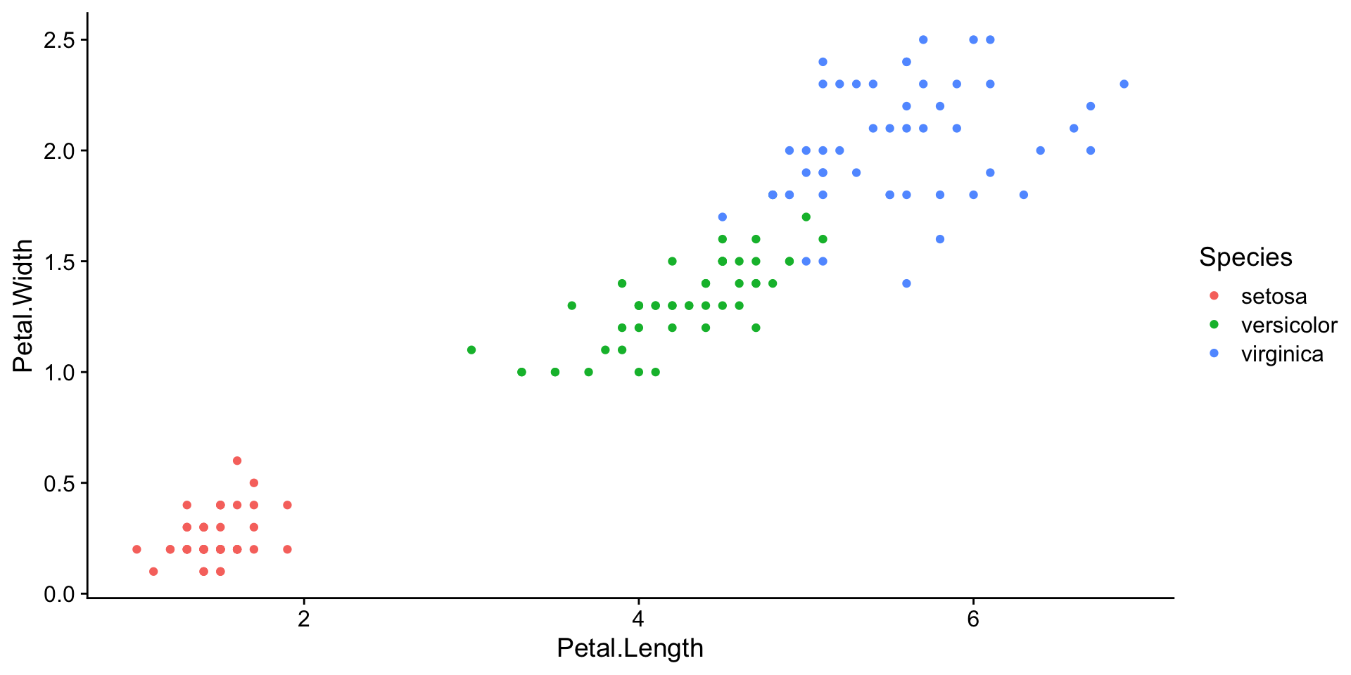
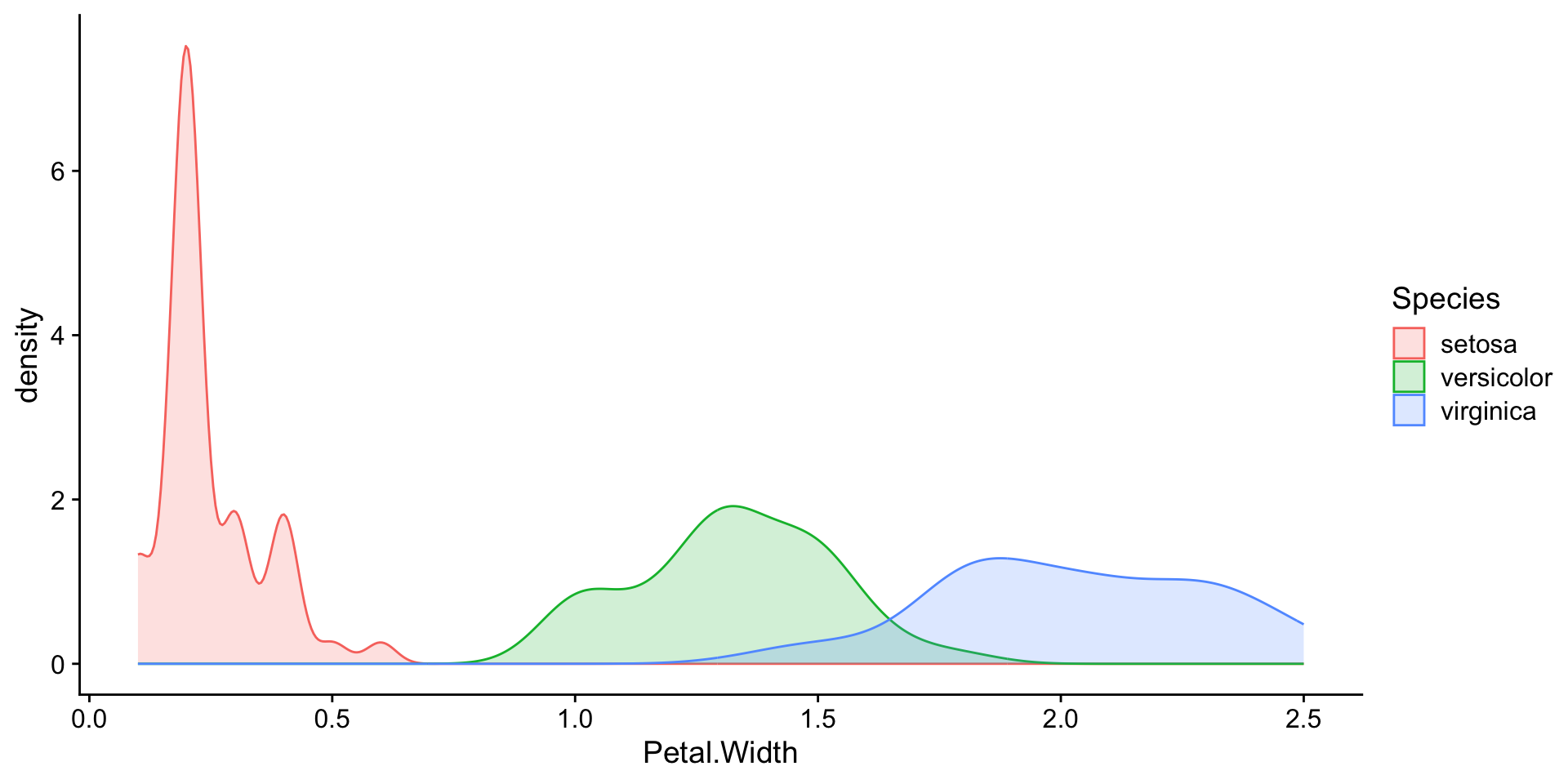
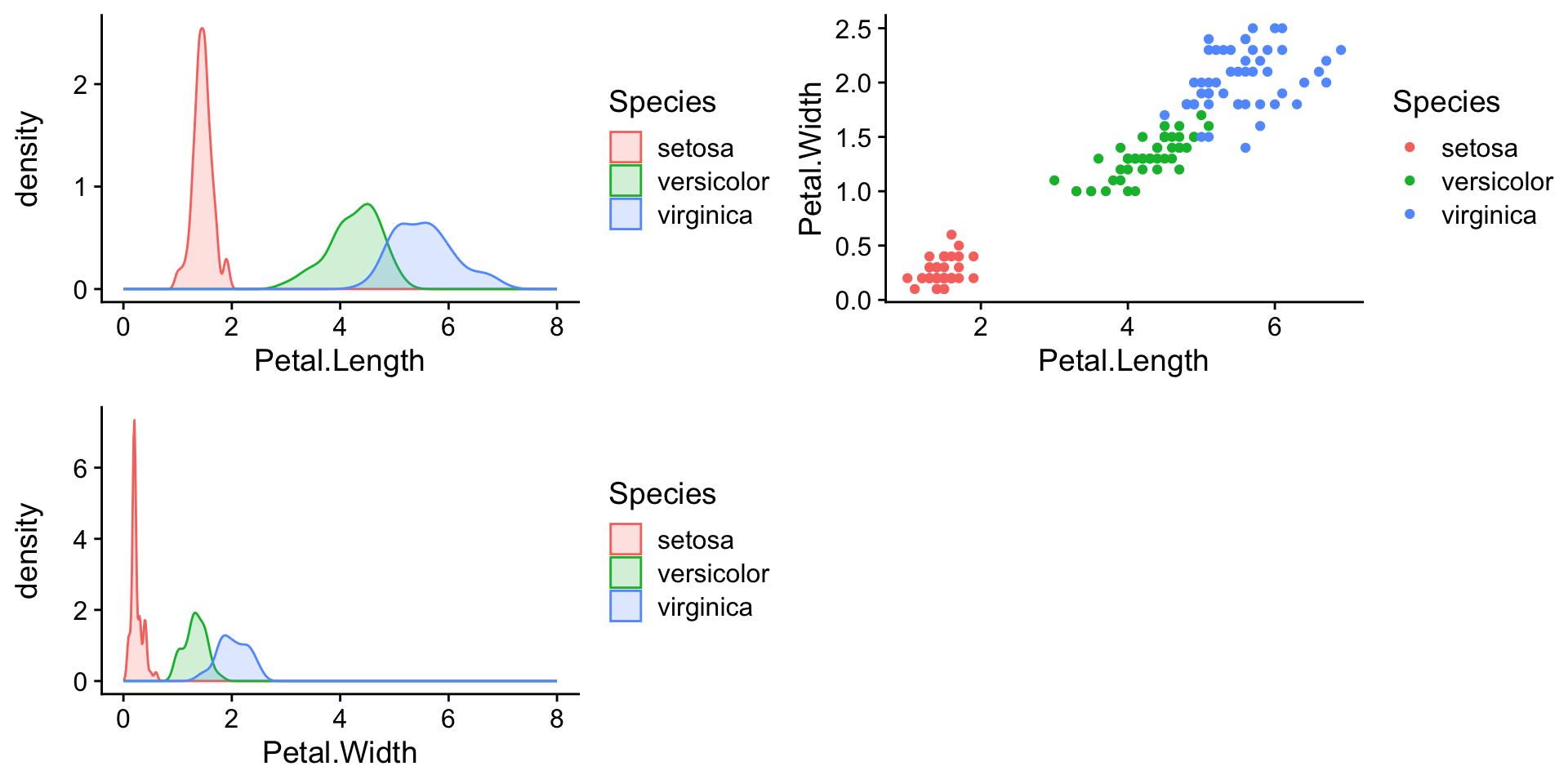
Shared legends
Plot overlays
iris_grid <- plot_grid(
plot_grid(
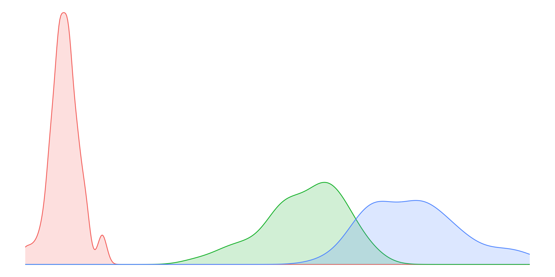
kde_length +
scale_x_continuous(limits = c(0,8)) +
theme(legend.position="none"),
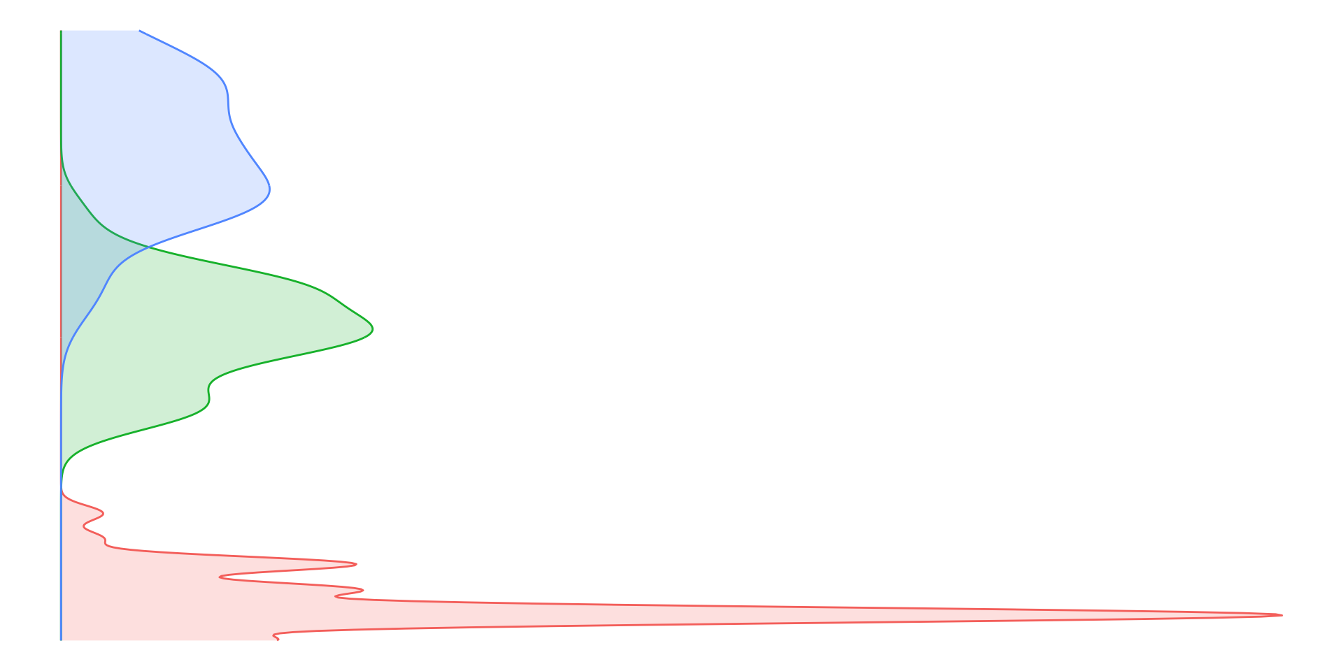
kde_width +
scale_x_continuous(limits = c(0,8)) +
theme(legend.position="none"),
ncol=1,
align="v"
),
scatter_petal +
theme(legend.position='none'),
ncol=2, rel_widths = c(1,2)
)
ggdraw(iris_grid) +
draw_grob(species_legend, x=0.8, y=-0.25)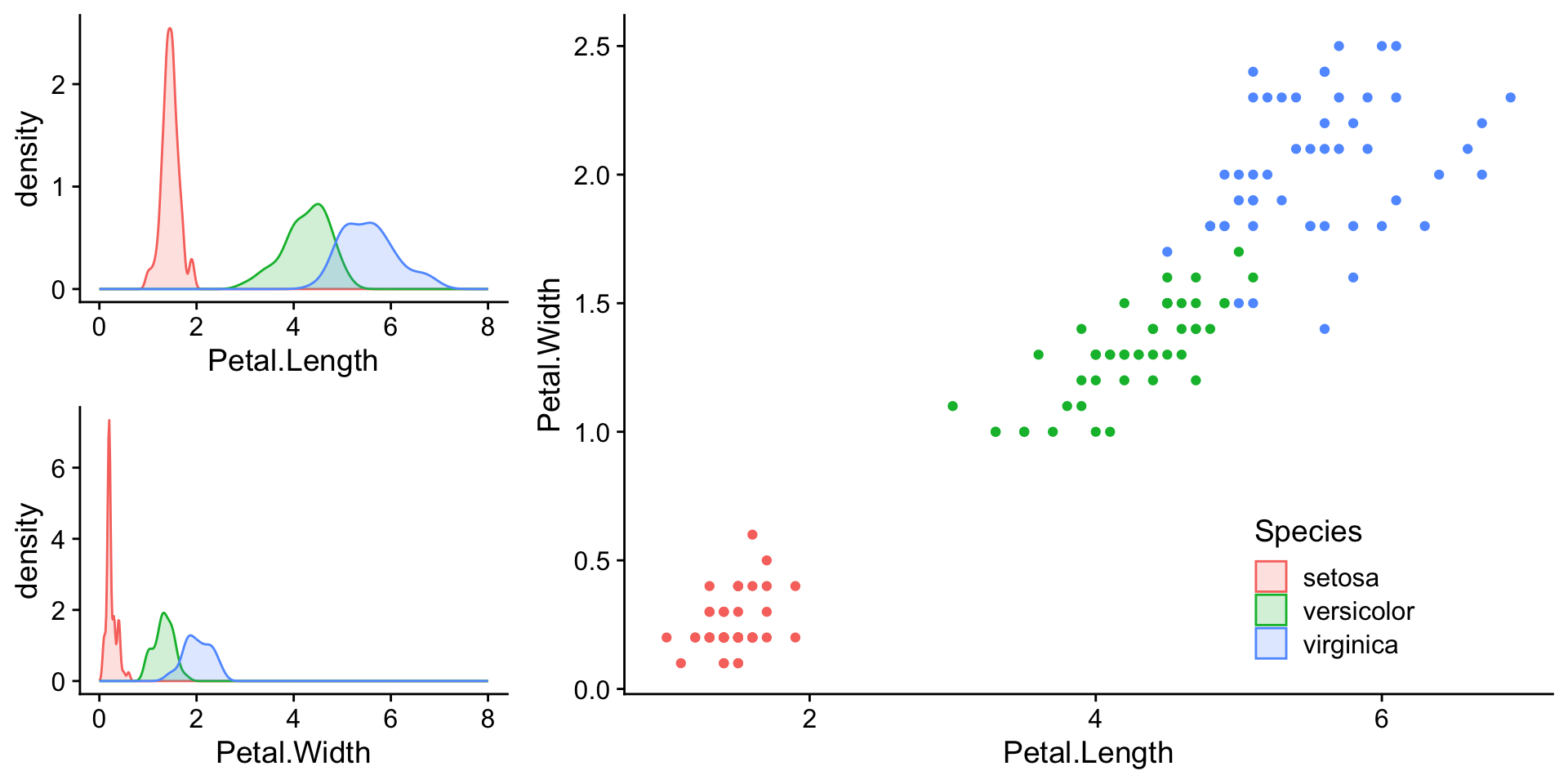
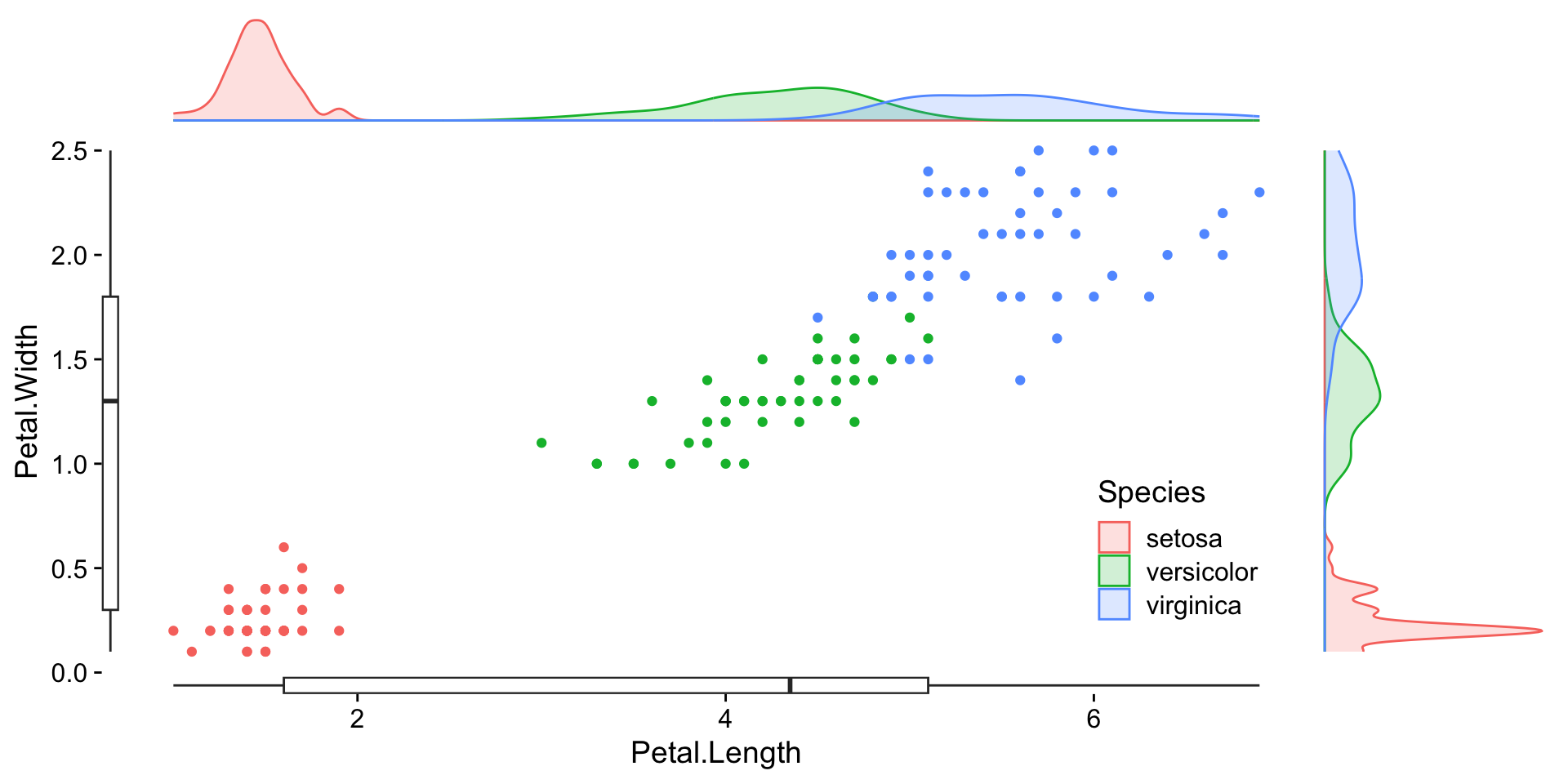
Margin plots
length_v <- kde_length +
  theme_void() +
  theme(legend.position="none")
width_v <- kde_width +
  coord_flip() +
  theme_void() +
  theme(legend.position="none")

p1 <- insert_xaxis_grob(
  scatter_petal +
    theme(legend.position = "none"),
  length_v, position="top")
p2 <- insert_yaxis_grob(
  p1, width_v,
  position="right")

ggdraw(p2) +
  draw_grob(species_legend, x=0.15, y=0.15)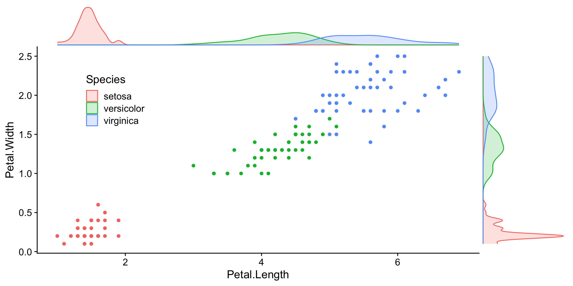
Margin plots