Data preprocessing

Data Visualization and Exploration

Ozan Kahramanoğulları

File reading

Data formats

There are several formats in which you can find data.

They can be broadly classified in two classes.

Textual data

human readable

often easy to parse

inter-operable in different environments

slow

may waste space (but compression helps)

Binary data

fast

compact

requires specialized software to be read

harder to access in different environments

not human readable

Comma Separated Values (CSV)

Textual data

One of the simplest textual formats

state, year, energy
DE, 2015, 8.803
IT, 2015, 9.879
DE, 2016, 8.917
IT, 2016, 10.062

library(tidyverse)

read_csv("data/example.csv")

# A tibble: 4 × 3
  state  year energy
  <chr> <dbl>  <dbl>
1 DE     2015   8.70
2 IT     2015   9.88
3 DE     2016   8.83
4 IT     2016  10.1

CSV’s friends

The delimiter separating symbol is not always a comma.

read_csv
read_tsv
read_delim

Missing values in the input

Input file:

state,year,energy
DE,2015,8.803
IT,2015,
DE,:,8.917
IT,2016,10.062

read_csv("data/example_na.csv", 
         na=c("", ":"))

# A tibble: 4 × 3
  state  year energy
  <chr> <dbl>  <dbl>
1 DE     2015   8.80
2 IT     2015  NA   
3 DE       NA   8.92
4 IT     2016  10.1

Specifying column names

This file does not have a header row!

DE,2015,8.803
IT,2015,9.879
DE,2016,8.917
IT,2016,10.062

read_csv(
  "data/example_no_names.csv",
)

# A tibble: 3 × 3
  DE    `2015` `8.803`
  <chr>  <dbl>   <dbl>
1 IT      2015    9.88
2 DE      2016    8.92
3 IT      2016   10.1

Specifying column names

We should specify the names manually

DE,2015,8.803
IT,2015,9.879
DE,2016,8.917
IT,2016,10.062

read_csv(
  "data/example_no_names.csv",
   col_names = c(
     "state", 
     "year", 
     "energy"
   )
)

# A tibble: 4 × 3
  state  year energy
  <chr> <dbl>  <dbl>
1 DE     2015   8.80
2 IT     2015   9.88
3 DE     2016   8.92
4 IT     2016  10.1

Data frames

A way of representing data

A data frame is the most common way to represent tabular data in R.
A data frame is essentially a list of vectors.
A data frame has
- several columns with names,
- many rows.

Processing data frames

Usually, you do not manipulate single values directly.
Instead, entire columns are processed all in one go.

`tibbles`

A tibble is an enhanced data frame with

better printing,
better type handling,
better defaults for building and subsetting,
and possibility to use invalid identifiers as column names.

Our running example

We will use a tibble of all the flights leaving the New Your airport in 2013.

renv::install("nycflights13")

This package contains 5 datasets.

nycflights13::airlines
nycflights13::airports
nycflights13::flights
nycflights13::planes
nycflights13::weather

We can easily inspect this using:

View(nycflights13::flights)

Our running example

# A tibble: 336,776 × 19
    year month   day dep_time sched_dep_time dep_delay arr_time sched_arr_time
   <int> <int> <int>    <int>          <int>     <dbl>    <int>          <int>
 1  2013     1     1      517            515         2      830            819
 2  2013     1     1      533            529         4      850            830
 3  2013     1     1      542            540         2      923            850
 4  2013     1     1      544            545        -1     1004           1022
 5  2013     1     1      554            600        -6      812            837
 6  2013     1     1      554            558        -4      740            728
 7  2013     1     1      555            600        -5      913            854
 8  2013     1     1      557            600        -3      709            723
 9  2013     1     1      557            600        -3      838            846
10  2013     1     1      558            600        -2      753            745
# ℹ 336,766 more rows
# ℹ 11 more variables: arr_delay <dbl>, carrier <chr>, flight <int>,
#   tailnum <chr>, origin <chr>, dest <chr>, air_time <dbl>, distance <dbl>,
#   hour <dbl>, minute <dbl>, time_hour <dttm>

Using `dplyr`

Dplyr

The dplyr library is part of the tidyverse.
It provides a consistent set of functions to solve most data manipulation problems.

But I came here for doing visualizations!

Data rarely comes in a readily usable form.

This means that we first need to know how to properly “prepare” the data.

General structure of a `dplyr` call

Usually you will bring all the functions of dplyr in scope using either

library(dplyr)

library(tidyverse)

The call to many dplyr functions looks like this:

function_name(data_frame, ...other arguments...)

In ...other arguments... you can refer to column names!

Filtering rows

filter(flights, month == 1, day == 1)

# A tibble: 842 × 19
    year month   day dep_time sched_dep_time dep_delay arr_time sched_arr_time
   <int> <int> <int>    <int>          <int>     <dbl>    <int>          <int>
 1  2013     1     1      517            515         2      830            819
 2  2013     1     1      533            529         4      850            830
 3  2013     1     1      542            540         2      923            850
 4  2013     1     1      544            545        -1     1004           1022
 5  2013     1     1      554            600        -6      812            837
 6  2013     1     1      554            558        -4      740            728
 7  2013     1     1      555            600        -5      913            854
 8  2013     1     1      557            600        -3      709            723
 9  2013     1     1      557            600        -3      838            846
10  2013     1     1      558            600        -2      753            745
# ℹ 832 more rows
# ℹ 11 more variables: arr_delay <dbl>, carrier <chr>, flight <int>,
#   tailnum <chr>, origin <chr>, dest <chr>, air_time <dbl>, distance <dbl>,
#   hour <dbl>, minute <dbl>, time_hour <dttm>

Filtering rows

How can we filter all the flights where the delay was less than 10?

How can we filter all the flights with missing departure delay?

Sorting data

arrange(flights, dep_delay)

# A tibble: 336,776 × 19
    year month   day dep_time sched_dep_time dep_delay arr_time sched_arr_time
   <int> <int> <int>    <int>          <int>     <dbl>    <int>          <int>
 1  2013    12     7     2040           2123       -43       40           2352
 2  2013     2     3     2022           2055       -33     2240           2338
 3  2013    11    10     1408           1440       -32     1549           1559
 4  2013     1    11     1900           1930       -30     2233           2243
 5  2013     1    29     1703           1730       -27     1947           1957
 6  2013     8     9      729            755       -26     1002            955
 7  2013    10    23     1907           1932       -25     2143           2143
 8  2013     3    30     2030           2055       -25     2213           2250
 9  2013     3     2     1431           1455       -24     1601           1631
10  2013     5     5      934            958       -24     1225           1309
# ℹ 336,766 more rows
# ℹ 11 more variables: arr_delay <dbl>, carrier <chr>, flight <int>,
#   tailnum <chr>, origin <chr>, dest <chr>, air_time <dbl>, distance <dbl>,
#   hour <dbl>, minute <dbl>, time_hour <dttm>

Sorting data

arrange(flights, desc(dep_delay))

# A tibble: 336,776 × 19
    year month   day dep_time sched_dep_time dep_delay arr_time sched_arr_time
   <int> <int> <int>    <int>          <int>     <dbl>    <int>          <int>
 1  2013     1     9      641            900      1301     1242           1530
 2  2013     6    15     1432           1935      1137     1607           2120
 3  2013     1    10     1121           1635      1126     1239           1810
 4  2013     9    20     1139           1845      1014     1457           2210
 5  2013     7    22      845           1600      1005     1044           1815
 6  2013     4    10     1100           1900       960     1342           2211
 7  2013     3    17     2321            810       911      135           1020
 8  2013     6    27      959           1900       899     1236           2226
 9  2013     7    22     2257            759       898      121           1026
10  2013    12     5      756           1700       896     1058           2020
# ℹ 336,766 more rows
# ℹ 11 more variables: arr_delay <dbl>, carrier <chr>, flight <int>,
#   tailnum <chr>, origin <chr>, dest <chr>, air_time <dbl>, distance <dbl>,
#   hour <dbl>, minute <dbl>, time_hour <dttm>

Getting column names

names(flights)

 [1] "year"           "month"          "day"            "dep_time"      
 [5] "sched_dep_time" "dep_delay"      "arr_time"       "sched_arr_time"
 [9] "arr_delay"      "carrier"        "flight"         "tailnum"       
[13] "origin"         "dest"           "air_time"       "distance"      
[17] "hour"           "minute"         "time_hour"

Selecting columns

select(flights, day, tailnum, distance)

# A tibble: 336,776 × 3
     day tailnum distance
   <int> <chr>      <dbl>
 1     1 N14228      1400
 2     1 N24211      1416
 3     1 N619AA      1089
 4     1 N804JB      1576
 5     1 N668DN       762
 6     1 N39463       719
 7     1 N516JB      1065
 8     1 N829AS       229
 9     1 N593JB       944
10     1 N3ALAA       733
# ℹ 336,766 more rows

Renaming columns

rename(flights, tail_num = tailnum)

# A tibble: 336,776 × 19
    year month   day dep_time sched_dep_time dep_delay arr_time sched_arr_time
   <int> <int> <int>    <int>          <int>     <dbl>    <int>          <int>
 1  2013     1     1      517            515         2      830            819
 2  2013     1     1      533            529         4      850            830
 3  2013     1     1      542            540         2      923            850
 4  2013     1     1      544            545        -1     1004           1022
 5  2013     1     1      554            600        -6      812            837
 6  2013     1     1      554            558        -4      740            728
 7  2013     1     1      555            600        -5      913            854
 8  2013     1     1      557            600        -3      709            723
 9  2013     1     1      557            600        -3      838            846
10  2013     1     1      558            600        -2      753            745
# ℹ 336,766 more rows
# ℹ 11 more variables: arr_delay <dbl>, carrier <chr>, flight <int>,
#   tail_num <chr>, origin <chr>, dest <chr>, air_time <dbl>, distance <dbl>,
#   hour <dbl>, minute <dbl>, time_hour <dttm>

Creating new columns

speed_data <- select(flights, distance, air_time)
mutate(speed_data, speed = distance * 60/ air_time)

# A tibble: 336,776 × 3
   distance air_time speed
      <dbl>    <dbl> <dbl>
 1     1400      227  370.
 2     1416      227  374.
 3     1089      160  408.
 4     1576      183  517.
 5      762      116  394.
 6      719      150  288.
 7     1065      158  404.
 8      229       53  259.
 9      944      140  405.
10      733      138  319.
# ℹ 336,766 more rows

Creating new columns

How can we add a column with the logarithm of the distance?

Conditional mutation

if_else( condition, value_if_true, value_if_false )

mutate(flights, 
       delayed_str = if_else(dep_delay > 0, "delayed", "not_delayed"))

# A tibble: 336,776 × 20
  dep_delay delayed_str  year month   day dep_time sched_dep_time arr_time
      <dbl> <chr>       <int> <int> <int>    <int>          <int>    <int>
1         2 delayed      2013     1     1      517            515      830
2         4 delayed      2013     1     1      533            529      850
3         2 delayed      2013     1     1      542            540      923
4        -1 not_delayed  2013     1     1      544            545     1004
5        -6 not_delayed  2013     1     1      554            600      812
# ℹ 336,771 more rows
# ℹ 12 more variables: sched_arr_time <int>, arr_delay <dbl>, carrier <chr>,
#   flight <int>, tailnum <chr>, origin <chr>, dest <chr>, air_time <dbl>,
#   distance <dbl>, hour <dbl>, minute <dbl>, time_hour <dttm>

Counting

count(flights)

# A tibble: 1 × 1
       n
   <int>
1 336776

count(flights, month)

# A tibble: 12 × 2
   month     n
   <int> <int>
 1     1 27004
 2     2 24951
 3     3 28834
 4     4 28330
 5     5 28796
 6     6 28243
 7     7 29425
 8     8 29327
 9     9 27574
10    10 28889
11    11 27268
12    12 28135

Summarising

summarise(flights, avg_delay = mean(dep_delay, na.rm = TRUE))

# A tibble: 1 × 1
  avg_delay
      <dbl>
1      12.6

summarise(flights, n_elems = n())

# A tibble: 1 × 1
  n_elems
    <int>
1  336776

More useful summarisation with `group_by`

grouped_flights <- group_by(flights, year, month)
summarise(grouped_flights, avg_delay = mean(dep_delay, na.rm = TRUE))

# A tibble: 12 × 3
# Groups:   year [1]
    year month avg_delay
   <int> <int>     <dbl>
 1  2013     1     10.0 
 2  2013     2     10.8 
 3  2013     3     13.2 
 4  2013     4     13.9 
 5  2013     5     13.0 
 6  2013     6     20.8 
 7  2013     7     21.7 
 8  2013     8     12.6 
 9  2013     9      6.72
10  2013    10      6.24
11  2013    11      5.44
12  2013    12     16.6

Summarisation

How can we get the maximum and minimum delay by year and month?

grouped_flights <- group_by(
  flights, year, month
)

summarise(
  grouped_flights, 
  max_delay = max(dep_delay, 
                  na.rm = TRUE),
  min_delay = min(dep_delay, 
                  na.rm = TRUE),
)

# A tibble: 12 × 4
# Groups:   year [1]
    year month max_delay min_delay
   <int> <int>     <dbl>     <dbl>
 1  2013     1      1301       -30
 2  2013     2       853       -33
 3  2013     3       911       -25
 4  2013     4       960       -21
 5  2013     5       878       -24
 6  2013     6      1137       -21
 7  2013     7      1005       -22
 8  2013     8       520       -26
 9  2013     9      1014       -24
10  2013    10       702       -25
11  2013    11       798       -32
12  2013    12       896       -43

Group by

The group_by function produces a grouped tibble.

This means that the operations applied on it act on each group separately.

How can you replicate the behavior of count(flights, month) using group_by, summarise, and n()?

grouped_flights <- group_by(
  flights, month
)

summarise(
  grouped_flights, 
  count = n()
)

# A tibble: 12 × 2
   month count
   <int> <int>
 1     1 27004
 2     2 24951
 3     3 28834
 4     4 28330
 5     5 28796
 6     6 28243
 7     7 29425
 8     8 29327
 9     9 27574
10    10 28889
11    11 27268
12    12 28135

Piping!

Instead of repeatedly assigning the result of each function to a variable that will be used just once, you can use the %>% operator

This operator takes the result of the function on its left
and
makes it the first argument of the function on its right.

Piping example

flights %>%
  select(month, distance, air_time) %>%
  mutate(speed = distance / air_time * 60) %>%
  group_by(month) %>%
  summarise(avg_speed = mean(speed, na.rm=TRUE))

# A tibble: 12 × 2
   month avg_speed
   <int>     <dbl>
 1     1      370.
 2     2      375.
 3     3      390.
 4     4      389.
 5     5      407.
 6     6      404.
 7     7      412.
 8     8      408.
 9     9      414.
10    10      397.
11    11      385.
12    12      377.

Joining two data frames

Sometimes the information we need is in different data frames and we need to join them.
This is a family of operations borrowed from the database world.
The basic idea:

we use the values taken by some columns in one table
to match rows in the other table.

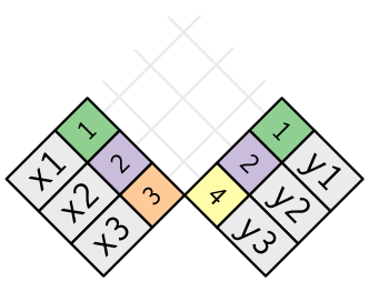
Join types

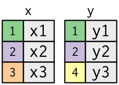
Two columns each: key (coloured) and value (gray)

Join types

x <- tibble(key=c(1,2,3),val_x=c("x1","x2","x3"))
x

# A tibble: 3 × 2
    key val_x
  <dbl> <chr>
1     1 x1   
2     2 x2   
3     3 x3

x <- tribble(
  ~key, ~val_x,
     1, "x1",
     2, "x2",
     3, "x3"
)

y <- tibble(key=c(1,2,4),val_x=c("y1","y2","y4"))
y

# A tibble: 3 × 2
    key val_x
  <dbl> <chr>
1     1 y1   
2     2 y2   
3     4 y4

y <- tribble(
  ~key, ~val_y,
     1, "y1",
     2, "y2",
     4, "y3" 
)

Join types

Join types: inner join

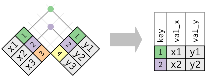
Keep only the rows that have keys in both tables

Join types: outer join

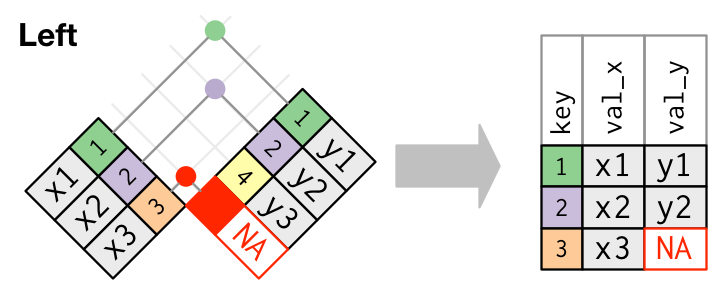
Keep all the rows from left table

Join types: outer join

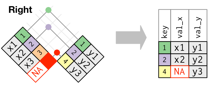
Keep all the rows from right table

Join types: outer join

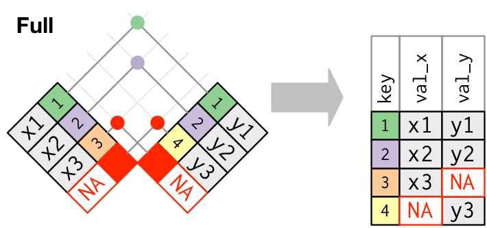
Keep all the rows from both tables

Join: duplicate keys

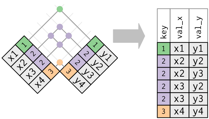
For a given key, get all the possible combinations of values

Join examples

inner_join(x,y, by="key")

# A tibble: 2 × 3
    key val_x.x val_x.y
  <dbl> <chr>   <chr>  
1     1 x1      y1     
2     2 x2      y2

# A tibble: 3 × 2
    key val_x
  <dbl> <chr>
1     1 x1   
2     2 x2   
3     3 x3

# A tibble: 3 × 2
    key val_x
  <dbl> <chr>
1     1 y1   
2     2 y2   
3     4 y4

Join examples

left_join(x,y, by="key")

# A tibble: 3 × 3
    key val_x.x val_x.y
  <dbl> <chr>   <chr>  
1     1 x1      y1     
2     2 x2      y2     
3     3 x3      <NA>

# A tibble: 3 × 2
    key val_x
  <dbl> <chr>
1     1 x1   
2     2 x2   
3     3 x3

# A tibble: 3 × 2
    key val_x
  <dbl> <chr>
1     1 y1   
2     2 y2   
3     4 y4

Join examples

right_join(x,y, by="key")

# A tibble: 3 × 3
    key val_x.x val_x.y
  <dbl> <chr>   <chr>  
1     1 x1      y1     
2     2 x2      y2     
3     4 <NA>    y4

# A tibble: 3 × 2
    key val_x
  <dbl> <chr>
1     1 x1   
2     2 x2   
3     3 x3

# A tibble: 3 × 2
    key val_x
  <dbl> <chr>
1     1 y1   
2     2 y2   
3     4 y4

Join examples

full_join(x,y, by="key")

# A tibble: 4 × 3
    key val_x.x val_x.y
  <dbl> <chr>   <chr>  
1     1 x1      y1     
2     2 x2      y2     
3     3 x3      <NA>   
4     4 <NA>    y4

# A tibble: 3 × 2
    key val_x
  <dbl> <chr>
1     1 x1   
2     2 x2   
3     3 x3

# A tibble: 3 × 2
    key val_x
  <dbl> <chr>
1     1 y1   
2     2 y2   
3     4 y4

An example on real data

flights2 <- select(flights, year, origin, dest, tailnum)
planes2 <- select(planes, tailnum, year, manufacturer, model)
inner_join(flights2, planes2, by="tailnum")

# A tibble: 284,170 × 7
   year.x origin dest  tailnum year.y manufacturer     model      
    <int> <chr>  <chr> <chr>    <int> <chr>            <chr>      
 1   2013 EWR    IAH   N14228    1999 BOEING           737-824    
 2   2013 LGA    IAH   N24211    1998 BOEING           737-824    
 3   2013 JFK    MIA   N619AA    1990 BOEING           757-223    
 4   2013 JFK    BQN   N804JB    2012 AIRBUS           A320-232   
 5   2013 LGA    ATL   N668DN    1991 BOEING           757-232    
 6   2013 EWR    ORD   N39463    2012 BOEING           737-924ER  
 7   2013 EWR    FLL   N516JB    2000 AIRBUS INDUSTRIE A320-232   
 8   2013 LGA    IAD   N829AS    1998 CANADAIR         CL-600-2B19
 9   2013 JFK    MCO   N593JB    2004 AIRBUS           A320-232   
10   2013 JFK    PBI   N793JB    2011 AIRBUS           A320-232   
# ℹ 284,160 more rows

Wrap up

Come up with a way to compute the fraction of delayed flights per month.

Tools of the trade

filter
mutate
select
rename
if_else
count
n

group_by
summarise
inner_join
outer_join
left_join
right_join

https://rstudio.com/resources/cheatsheets/

Solution 1

all_counts <- flights %>%
  filter(!is.na(dep_delay)) %>%
  count(month)

delayed_flights <- flights %>%
  filter(!is.na(dep_delay)) %>%
  filter(dep_delay > 0) %>%
  count(month) %>%
  rename(n_delayed = n)

inner_join(delayed_flights, all_counts, 
           by="month") %>%
  mutate(
    fraction_delayed = n_delayed / n
  ) %>%
  select(month, fraction_delayed)

# A tibble: 12 × 2
   month fraction_delayed
   <int>            <dbl>
 1     1            0.365
 2     2            0.385
 3     3            0.401
 4     4            0.381
 5     5            0.400
 6     6            0.465
 7     7            0.488
 8     8            0.406
 9     9            0.288
10    10            0.304
11    11            0.305
12    12            0.500

Solution 2

flights %>% 
  filter(!is.na(dep_delay)) %>%
  select(month,dep_delay) %>% 
  group_by(month) %>% 
  summarise(delayed = sum(dep_delay>0),all=n()) %>% 
  mutate(fraction_delayed=delayed/all) %>%
  select(month,fraction_delayed)

# A tibble: 12 × 2
   month fraction_delayed
   <int>            <dbl>
 1     1            0.365
 2     2            0.385
 3     3            0.401
 4     4            0.381
 5     5            0.400
 6     6            0.465
 7     7            0.488
 8     8            0.406
 9     9            0.288
10    10            0.304
11    11            0.305
12    12            0.500

Solution 3

flights %>%
  mutate(is_delayed = if_else(dep_delay > 0, 1, 0)) %>%
  group_by(month) %>%
  filter(!is.na(is_delayed)) %>%
  summarise(fraction_delayed = sum(is_delayed) / n())

# A tibble: 12 × 2
   month fraction_delayed
   <int>            <dbl>
 1     1            0.365
 2     2            0.385
 3     3            0.401
 4     4            0.381
 5     5            0.400
 6     6            0.465
 7     7            0.488
 8     8            0.406
 9     9            0.288
10    10            0.304
11    11            0.305
12    12            0.500

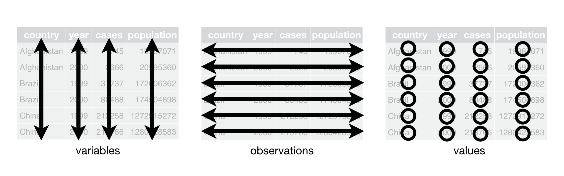
Tidy data

Each variable must have its own column.
Each observation must have its own row.
Each value must have its own cell.

A tidy data frame

Alarm bells

Column names that should be values.
Values that should be column names.

Making data tidy

Most datasets are not tidy

A variable might be spread across multiple columns.
An observation might be scattered across multiple rows.

We mainly have two tools to fix these two problems:

pivot_longer

pivot_wider

Example 1

Is this data frame tidy?

table4b

# A tibble: 3 × 3
  country         `1999`     `2000`
  <chr>            <dbl>      <dbl>
1 Afghanistan   19987071   20595360
2 Brazil       172006362  174504898
3 China       1272915272 1280428583

A variable might be spread across multiple columns.

Longer

pivot_longer(table4b, 
             `1999`:`2000`, 
             names_to = "year", 
             values_to = "population")

# A tibble: 6 × 3
  country     year  population
  <chr>       <chr>      <dbl>
1 Afghanistan 1999    19987071
2 Afghanistan 2000    20595360
3 Brazil      1999   172006362
4 Brazil      2000   174504898
5 China       1999  1272915272
6 China       2000  1280428583

Was:

# A tibble: 3 × 3
  country         `1999`     `2000`
  <chr>            <dbl>      <dbl>
1 Afghanistan   19987071   20595360
2 Brazil       172006362  174504898
3 China       1272915272 1280428583

Longer

Example 2

Is this data frame tidy?

table2

# A tibble: 12 × 4
   country      year type            count
   <chr>       <dbl> <chr>           <dbl>
 1 Afghanistan  1999 cases             745
 2 Afghanistan  1999 population   19987071
 3 Afghanistan  2000 cases            2666
 4 Afghanistan  2000 population   20595360
 5 Brazil       1999 cases           37737
 6 Brazil       1999 population  172006362
 7 Brazil       2000 cases           80488
 8 Brazil       2000 population  174504898
 9 China        1999 cases          212258
10 China        1999 population 1272915272
11 China        2000 cases          213766
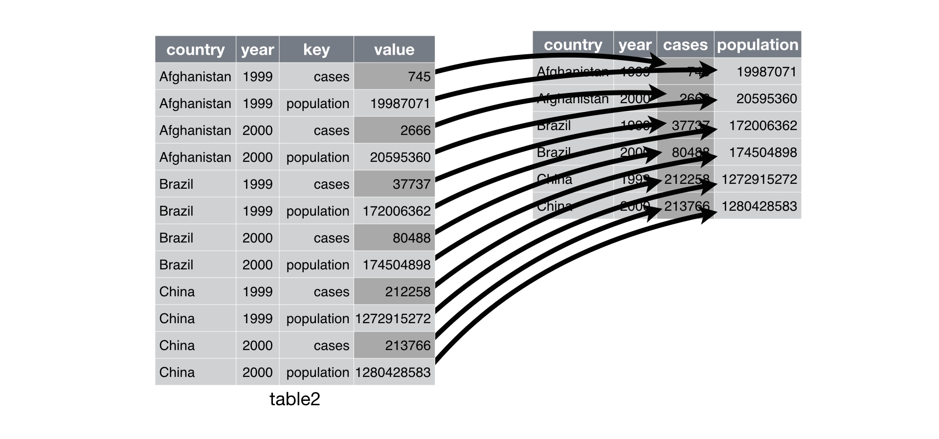
12 China        2000 population 1280428583

An observation might be scattered across multiple rows.

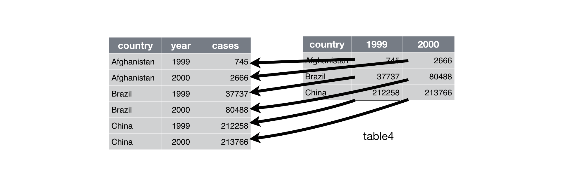
Wider

pivot_wider(table2, 
            names_from=type, 
            values_from=count)

# A tibble: 6 × 4
  country      year  cases population
  <chr>       <dbl>  <dbl>      <dbl>
1 Afghanistan  1999    745   19987071
2 Afghanistan  2000   2666   20595360
3 Brazil       1999  37737  172006362
4 Brazil       2000  80488  174504898
5 China        1999 212258 1272915272
6 China        2000 213766 1280428583

Was:

# A tibble: 12 × 4
   country      year type            count
   <chr>       <dbl> <chr>           <dbl>
 1 Afghanistan  1999 cases             745
 2 Afghanistan  1999 population   19987071
 3 Afghanistan  2000 cases            2666
 4 Afghanistan  2000 population   20595360
 5 Brazil       1999 cases           37737
 6 Brazil       1999 population  172006362
 7 Brazil       2000 cases           80488
 8 Brazil       2000 population  174504898
 9 China        1999 cases          212258
10 China        1999 population 1272915272
11 China        2000 cases          213766
12 China        2000 population 1280428583

Wider

Example 3

Is this table tidy?

table3

# A tibble: 6 × 3
  country      year rate             
  <chr>       <dbl> <chr>            
1 Afghanistan  1999 745/19987071     
2 Afghanistan  2000 2666/20595360    
3 Brazil       1999 37737/172006362  
4 Brazil       2000 80488/174504898  
5 China        1999 212258/1272915272
6 China        2000 213766/1280428583

Separating

separate(table3, 
         rate, 
         into = c("cases", "population"))

# A tibble: 6 × 4
  country      year cases  population
  <chr>       <dbl> <chr>  <chr>     
1 Afghanistan  1999 745    19987071  
2 Afghanistan  2000 2666   20595360  
3 Brazil       1999 37737  172006362 
4 Brazil       2000 80488  174504898 
5 China        1999 212258 1272915272
6 China        2000 213766 1280428583

Is there something odd?

Separating

separate(table3, 
         rate, 
         into = c("cases", "population"), 
         convert = TRUE)

# A tibble: 6 × 4
  country      year  cases population
  <chr>       <dbl>  <int>      <int>
1 Afghanistan  1999    745   19987071
2 Afghanistan  2000   2666   20595360
3 Brazil       1999  37737  172006362
4 Brazil       2000  80488  174504898
5 China        1999 212258 1272915272
6 China        2000 213766 1280428583

Separating

separate(table3, 
         rate, 
         into = c("cases", "population"), 
         convert = TRUE, 
         sep="/")

# A tibble: 6 × 4
  country      year  cases population
  <chr>       <dbl>  <int>      <int>
1 Afghanistan  1999    745   19987071
2 Afghanistan  2000   2666   20595360
3 Brazil       1999  37737  172006362
4 Brazil       2000  80488  174504898
5 China        1999 212258 1272915272
6 China        2000 213766 1280428583

A real-world example

Available from https://ec.europa.eu/eurostat/api/dissemination/sdmx/2.1/data/educ_uoe_grad05?format=tsv

freq,unit,isced11,age,geo\TIME_PERIOD   2013    2014    2015    2016    2017    2018    2019    2020    2021    2022 
A,P_THAB,ED5,TOTAL,AL   :   :   :   :   :   :   :   :   2.9     3.8 
A,P_THAB,ED5,TOTAL,AT   25.1    24.8    24.3    21.8    22.7    22.8    22.7    25.5    23.8    22.3 
A,P_THAB,ED5,TOTAL,BE   1.8     1.8     : d 2.1     2.1     2.0     2.0 d   3.8 d   5.1     4.9 
A,P_THAB,ED5,TOTAL,BG   : z : z : z : z : z : z : z : z : z : z
A,P_THAB,ED5,TOTAL,CH   2.2     1.9     0.5     0.4     0.3     0.3     0.3     0.3     0.4     : 
A,P_THAB,ED5,TOTAL,CY   7.3     7.5     6.9     7.0     6.4     7.8     7.1     7.4     9.1     7.8 
A,P_THAB,ED5,TOTAL,CZ   0.3     0.3     0.3     0.3     0.3     0.3     0.3     0.3     0.4     0.4

Discuss how to load this file into a tidy dataframe.

read_tsv(path, na, ....)
pivot_longer(data, columns, names_to=key, values_to=value)
pivot_wider(data, names_from=key, values_from=value)
separate(data, col, into, ...)

Cheat sheets

https://rstudio.com/resources/cheatsheets/

A real world example

education_data <- read_tsv("data/energy_productivity.tsv.gz", 
                                na=c("", ":"))

# A tibble: 78 × 21
  `unit,geo\\time` `2000` `2001` `2002` `2003` `2004` `2005` `2006` `2007`
  <chr>             <dbl>  <dbl>  <dbl>  <dbl>  <dbl>  <dbl>  <dbl>  <dbl>
1 EUR_KGOE,AT        8.69   8.34   8.43   8.08   8.15   8.06   8.26   8.72
2 EUR_KGOE,BA       NA     NA     NA     NA     NA     NA     NA     NA   
3 EUR_KGOE,BE        4.73   4.83   4.95   4.77   4.91   5.05   5.18   5.38
4 EUR_KGOE,BG        1.32   1.31   1.42   1.45   1.59   1.61   1.67   1.81
# ℹ 74 more rows
# ℹ 12 more variables: `2008` <dbl>, `2009` <dbl>, `2010` <dbl>, `2011` <dbl>,
#   `2012` <dbl>, `2013` <dbl>, `2014` <dbl>, `2015` <dbl>, `2016` <dbl>,
#   `2017` <dbl>, `2018` <dbl>, `2019` <dbl>

energy_productivity %>%
  pivot_longer(`2000`:`2019`, names_to='year', values_to='energy_productivity')

# A tibble: 1,560 × 3
   `unit,geo\\time` year  energy_productivity
   <chr>            <chr>               <dbl>
 1 EUR_KGOE,AT      2000                 8.69
 2 EUR_KGOE,AT      2001                 8.34
 3 EUR_KGOE,AT      2002                 8.43
 4 EUR_KGOE,AT      2003                 8.08
 5 EUR_KGOE,AT      2004                 8.15
 6 EUR_KGOE,AT      2005                 8.06
 7 EUR_KGOE,AT      2006                 8.26
 8 EUR_KGOE,AT      2007                 8.72
 9 EUR_KGOE,AT      2008                 8.78
10 EUR_KGOE,AT      2009                 8.90
# ℹ 1,550 more rows

energy_productivity %>%
  pivot_longer(`2000`:`2019`, names_to='year', values_to='energy_productivity') %>%
  separate(`unit,geo\\time`, into=c("unit", "state"), sep=',')

# A tibble: 1,560 × 4
   unit     state year  energy_productivity
   <chr>    <chr> <chr>               <dbl>
 1 EUR_KGOE AT    2000                 8.69
 2 EUR_KGOE AT    2001                 8.34
 3 EUR_KGOE AT    2002                 8.43
 4 EUR_KGOE AT    2003                 8.08
 5 EUR_KGOE AT    2004                 8.15
 6 EUR_KGOE AT    2005                 8.06
 7 EUR_KGOE AT    2006                 8.26
 8 EUR_KGOE AT    2007                 8.72
 9 EUR_KGOE AT    2008                 8.78
10 EUR_KGOE AT    2009                 8.90
# ℹ 1,550 more rows

Bonus: finding problematic values

If you have a dataframe with NA values, you can list them using the following snippet.

# This is the same dataset we used in the assignment
url_education <- "https://ec.europa.eu/eurostat/api/dissemination/sdmx/2.1/data/educ_uoe_grad05?format=tsv" 
# We load it from the file, dealing with the NA encodings we already know of
education_raw <- read_tsv(url_education,na=c(":",": z",": d"))  %>%
  mutate(across(everything(), as.character))
education_raw %>% 
  # Then we pivot the columns for more convenient processing
  pivot_longer(`2022`:`2013`, names_to="year", values_to="value") %>%
  # Once you find the problematic parts of the strings, you can uncomment the 
  # following line to remove the problematic characters
  #   mutate(value = str_remove(value, "d")) %>%
  # Here we keep only the values whose parsing results in a NA
  filter(is.na(as.double(value))) %>%
  # With distinct you remove the duplicates, getting an overview of the problematic values
  distinct(value)

# A tibble: 147 × 1
   value 
   <chr> 
 1 <NA>  
 2 3.8 d 
 3 2.0 d 
 4 8.6 d 
 5 7.7 d 
 6 9.3 d 
 7 8.0 d 
 8 21.9 d
 9 27.1 d
10 22.8 d
# ℹ 137 more rows

Data preprocessing

File reading

Data formats

Textual data

Binary data

Comma Separated Values (CSV)

Textual data

CSV’s friends

Missing values in the input

Specifying column names

Specifying column names

Data frames

A way of representing data

Processing data frames

tibbles

Our running example

Our running example

Using dplyr

Dplyr

General structure of a dplyr call

Filtering rows

Filtering rows

Sorting data

Sorting data

Getting column names

Selecting columns

Renaming columns

Creating new columns

Creating new columns

Conditional mutation

Counting

Summarising

More useful summarisation with group_by

Summarisation

Group by

Piping!

Piping example

Joining two data frames

Joining two data frames

Join types

Join types

Join types

Join types: inner join

Join types: outer join

Join types: outer join

Join types: outer join

Join: duplicate keys

Join examples

Join examples

Join examples

Join examples

An example on real data

Wrap up

Tools of the trade

Solution 1

Solution 2

Solution 3

Tidy data

Tidy data

A tidy data frame

Alarm bells

Making data tidy

Example 1

Longer

Longer

Example 2

Wider

Wider

Example 3

Separating

Separating

Separating

A real-world example

Cheat sheets

A real world example

Bonus: finding problematic values

`tibbles`

Using `dplyr`

General structure of a `dplyr` call

More useful summarisation with `group_by`