Introduction to R
Data Visualization and Exploration
The R programming language

R is a language and environment for statistical computing and graphics.
You will use it both for this course and for the Mathematics and Statistics course.
R: language overview
Some fundamental features
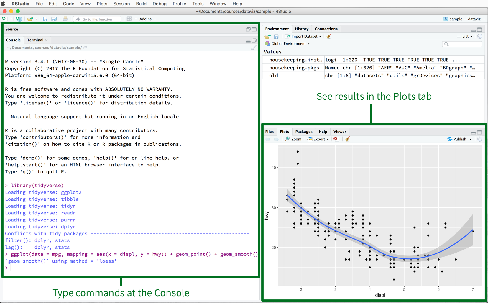
Interacting with the console
- Install RStudio: https://www.rstudio.com/products/rstudio/download/#download
Interacting with the console
- Install RStudio: https://www.rstudio.com/products/rstudio/download/#download
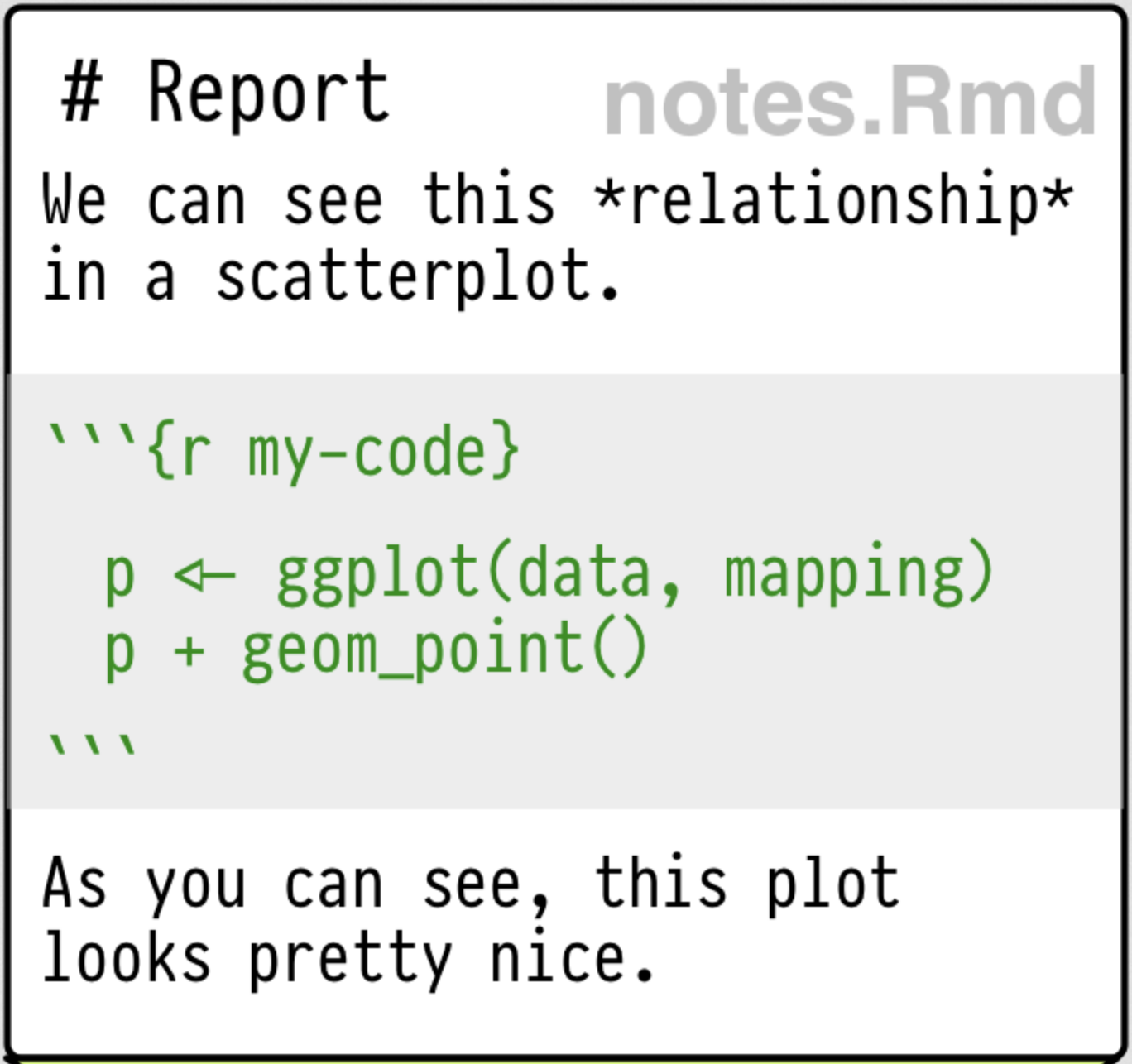
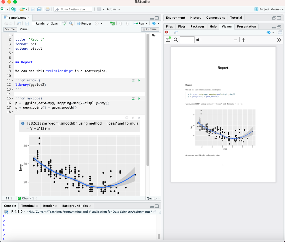
RMarkdown
RMarkdown is a plain text format (and accompanying tools) that allows you to intersperse text, code, and outputs.
obsolete
replaced with Quarto
(RMarkdown is integrated into Quarto)
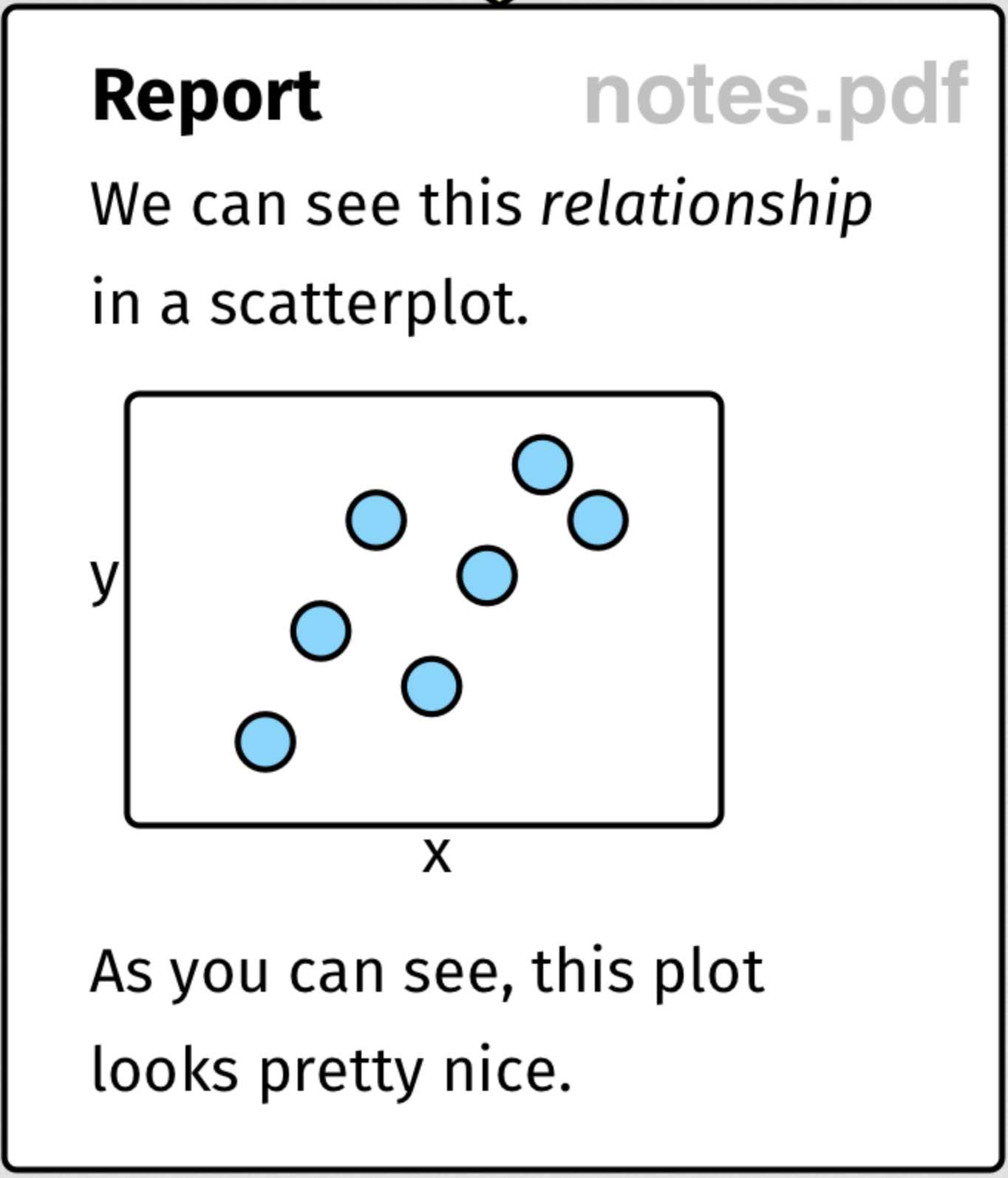
The RMarkdown pipeline
Advantages of RMarkdown Quarto
Keep analysis code together with discussion conclusions
Easily keep everything under version control
Reproducibility
Similar to Python’s notebooks
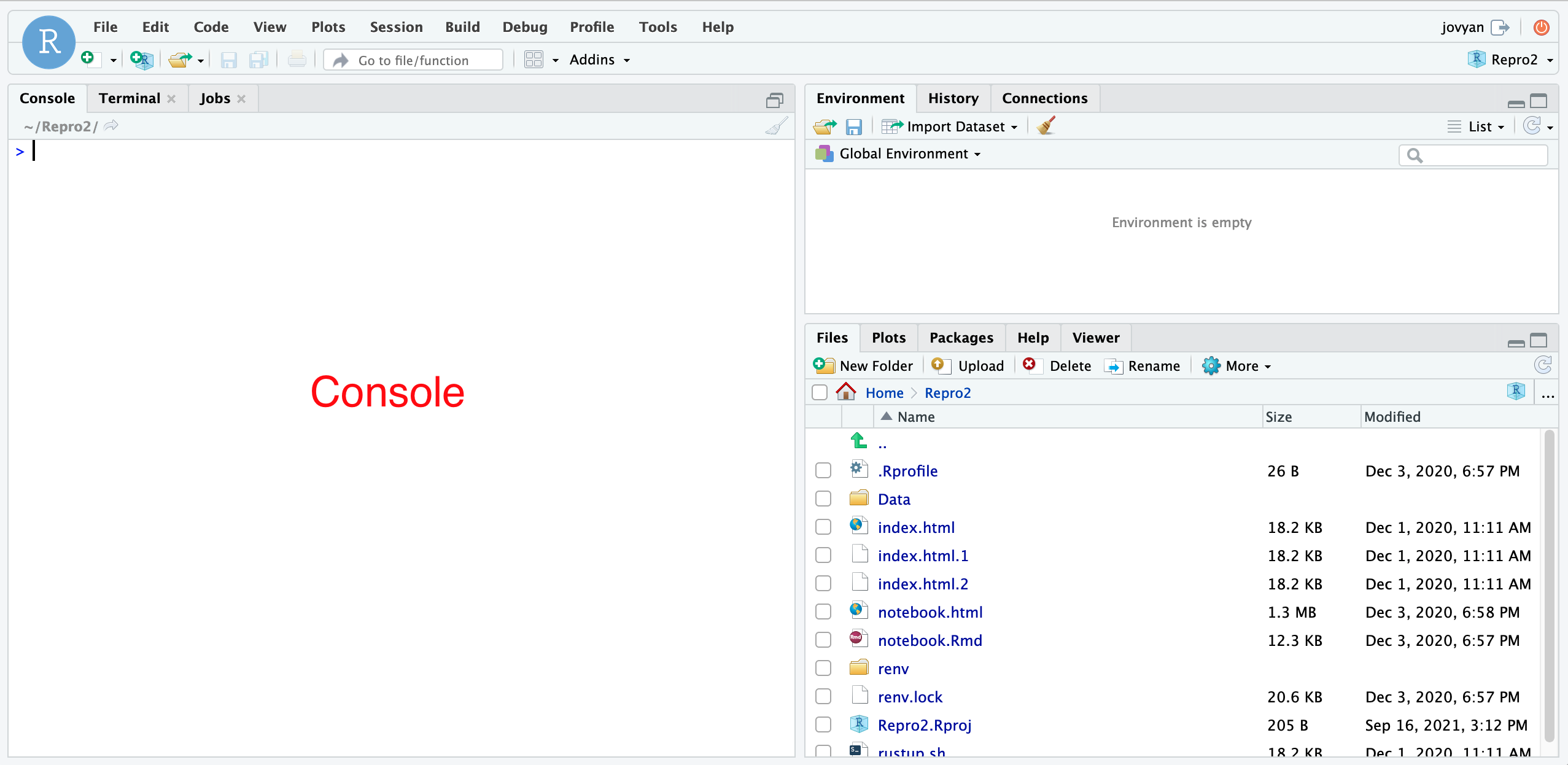
RStudio
R is an interpreter with which you interact using a text console.
You can use it in RStudio, an IDE with many features.
Built in console
Built in image viewer
Editor with auto-completion, syntax highlighting and all the nice things
Data types
R has five basic data types:
Names
In R, everything can be given a name.
x
# this is a valid name
descriptive_name
# descriptive names are preferable
# - note the underscore separating the words
# - spaces are not allowed
also.valid
# This is also a valid name, using an older and maybe
# confusing naming scheme. If you come from Java/C++/Python/Javascript....
# the . in the middle of the name is *not* the member access operator
These names (and others) are not allowed.
Some names are best avoided, because they are library functions that you would overwrite.
Binding things to names
Using the “arrow” syntax you can assign names to things.
Using R as a calculator
Arithmetic
Boolean values and comparisons
Using R as a calculator
What does the following comparison return (sqrt gives the square root)?
\[ (\sqrt{2})^2 = 2 \]
[1] FALSE
Missing values
The NA keyword represents a missing value.
[1] NA[1] NA[1] NAMissing values
To check if a value is NA you use the is.na function.
Other special values
What is the result of this operation?
[1] NaNThe NaN value (Not a Number): the result cannot be represented by a computer.
What about this operation?
[1] NaNWe get NaN even if this would be the definition of the complex number i.
If you want the complex number, then you should declare it explicitly.
NA vs NaN
Beware: in R the values NA and NaN refer to distinct concepts.
This is in contrast with Python, where NaN is often used also to indicate missing values.
Other special values
What about this operation?
[1] InfThe Inf value is used to represent infinity, and propagates in calculations.
[1] NaNVectors
Atomic vectors are homogeneous indexed collections of values of the same basic data type.
Vectors
You can ask for the type of a vector using typeof.
Vectors
You can ask for the length of a vector using length.
What about scalars?
What does this return?
[1] "double"[1] 1There are no scalar values, but vectors of length 1!
Vectors
The c function combines its arguments.
[1] 1 3 5 7 2 4 6 8Using c multiple times does not nest vectors
Vectors
What about this code?
[1] "1" "hello" "0.45" This is called implicit coercion.
It converts all the elements to the type that can represent all of them.
Coercion
Recycling

Recycling
What do you think will happen with this code?
[1] 2 3 4R coerces the length of vectors, if needed.
Remember that 1 is a vector of length one.
By coercion, in the operation above, it is replaced with c(1, 1, 1) by recycling its value.
So what about this?
[1] 2 5 4Operations on logical vectors
There are distinct operators for element-wise operators on logical vectors:
Operations on logical vectors
How can you check if all the values are FALSE?
Naming vectors
Elements of vectors can be named, which will be useful for indexing into the vector.
Notice that you need to enclose a name in quotes only if it contains spaces.
Subsetting vectors
You can index into vectors using integer indexes.
Beware: indexing starts from 1!
So what about this?
character(0)And this?
[1] NASubsetting vectors
Subsetting vectors
What does the code below give?
[1] "values" "these" [1] "these" "these" "some" "some" "these"Subsetting vectors
What about
[1] "these" "some" "values"Negative indices remove values from a vector!
Subsetting vectors
You can use boolean vectors to retain only the entries corresponding to TRUE.
Subsetting and naming
Is the following naming valid?
Subsetting and naming
Is the following naming valid?
This is not valid, since it makes subsetting ambiguous.
Heterogeneous collections
A list allows to store elements of different type in the same collection, without coercion.
Named, nested lists
Looking at the structure of nested lists
With the str function you can look at the structure of nested lists.
Going to higher dimensions: matrix
R support matrices out of the box. The following matrix
\[ \left[ \begin{matrix} 1 & 3 \\ 2 & 4 \end{matrix} \right] \]
can be specified as follows.
Transposing and concatenating
Consider the following two matrices.
Indexing matrices
Linear algebra operations on matrices
Control flow
Control flow: if
Control flow: for loops
We will use the following data as examples.
List of 4
 $ a: num [1:10] -1.207 0.277 1.084 -2.346 0.429 ...
 $ b: num [1:10] 0.317 0.303 0.159 0.04 0.219 ...
 $ c: num [1:10] 0.877 0.0146 1.8351 0.5193 1.9963 ...
 $ d: num [1:10] -159.354 -1.608 21.193 0.963 -0.907 ...
Control flow: for loops
We want to compute the mean of each of a, b, c and d in loop_data.
A straighforward approach would be
data_means <- list(
  a = mean(loop_data$a),
  b = mean(loop_data$b),
  c = mean(loop_data$c),
  d = mean(loop_data$d)
)
str(data_means)
List of 4
$ a: num -0.383
$ b: num 0.417
$ c: num 0.855
$ d: num -20.9What are the issues with this approach?
- Much repetition
- We must modify the code if we ever extend the list.
Control flow: for loops
We can do better with a for loop
data_means <- list()
for (i in 1:length(loop_data)) {
  data_means <- c(
    data_means,
    mean(loop_data[[i]])
  )
}

str(data_means)
List of 4
$ : num -0.383
$ : num 0.417
$ : num 0.855
$ : num -20.9Did we lose something?
Control flow: for loops
Functions
Functions
Whenever you find yourself copy-pasting the code, create a function instead!
The name of the function serves to describe its purpose.
Maintenance is easier: you only need to update code in one place.
You don’t make silly copy-paste errors.
Functions: anatomy
Function call
Functions: an example
Consider the following data
List of 4
 $ a: num [1:5] 0.00986 0.67827 1.02956 -1.72953 -2.20435
 $ b: num [1:5] -1.319 1.453 -37.231 0.164 -4.862
 $ c: num [1:5] 0.1215 0.8928 0.0146 0.7831 0.09
 $ d: num [1:5] 0.0384 1.2302 2.2003 0.9757 0.337
we want to rescale all the values so that they lie in the range 0 to 1.
Functions: an example
Let’s first see how to do it on my_list$a:
Functions: an example
Now, instead of copying and pasting the code for all the entries in my_list,
we define a function rescale01
and then we can invoke it, maybe in a loop.
Functions: variable number of arguments
You can write functions that accept a variable number of arguments using the ... syntax:
Libraries
Libraries
The tidyverse
Using libraries
Using libraries
The second option is more convenient.
However, some names may mask the names already in scope.
Renv
Helping with reproducibility
Scenario
Imagine the following situation.
You install some libraries.
You develop a program using those libraries.
You send the program to someone else.
The program breaks in mysterious and subtle ways.

Scenario 2
Imagine the following situation.
You install some libraries.
You develop a program using those libraries.
You start a new project, for which you need an updated version of the libraries.
After a while, you go back to your first project, and it’s broken in mysterious and sublte ways!

Problems
- Libraries change the way they work from one version to the other.
- To get consistent results:
- be explicit about their versions;
- isolate projects.
install.packagesby itself is not enough:- always installs the latest version;
- installed packages are shared between all projects.
Renv to the rescue!
renv(for Reproducible environments) is a system to manage dependencies in a saner way.It allows you to install your dependencies inside your working directory.
- Your project now contains:
- your code,
- all your dependencies.
You can share this bundle with others and they will be able to build an exact copy of your environment.
All your projects can depend on different versions of the same libraries.
Using renv
Restore missing libraries.
This is run automatically when you open a renv-managed project.
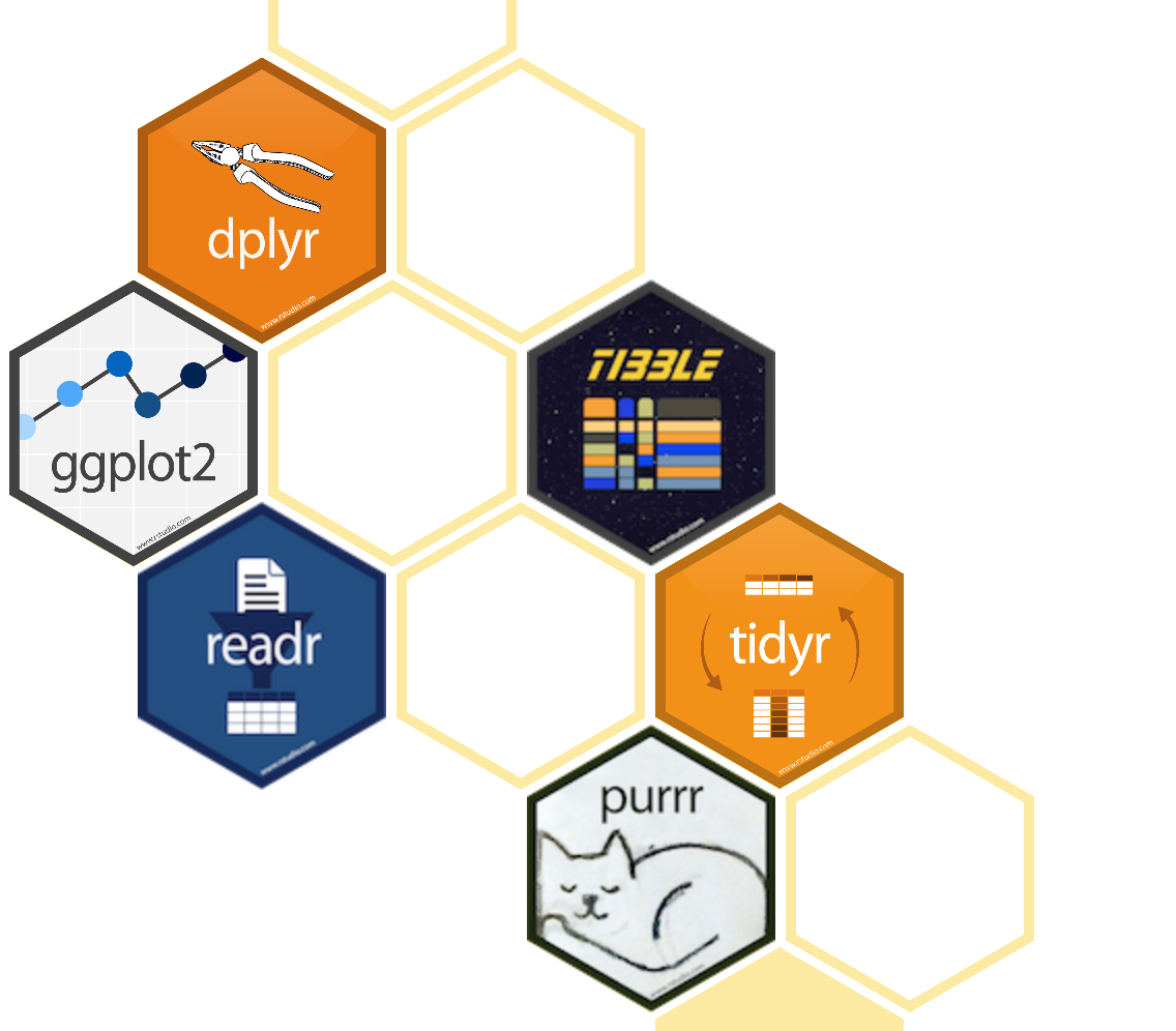
The Tidyverse libraries
The Tidyverse
The tidyverse is an opinionated collection of R packages designed for data science. All packages share an underlying design philosophy, grammar, and data structures.
The main library we will deal with.
Declarative graphics with a well-defined grammar.
The main reason we use R rather than python.
![]()
The tabular data representation we will mostly use.
A modern iteration on the data frame concept.

Data manipulation library.
Covers most of our preprocessing needs.
Reads a variety of file formats in a convenient way.
Handles corner cases and encodings for you.
Data Visualization and Exploration - Introduction to R - ozan-k.com